Render Engineering
APIs
Graphics APIs
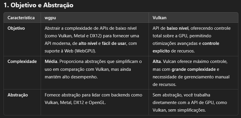
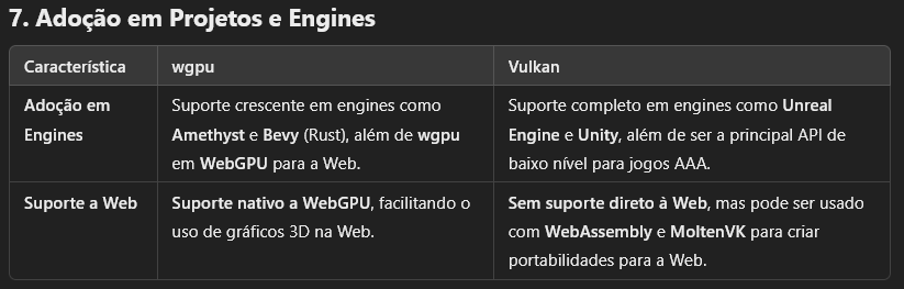
Vulkan
-
Vulkan .
-
Open Source Open Standard.
-
Type:
-
Low-level graphics API
-
-
Platforms:
-
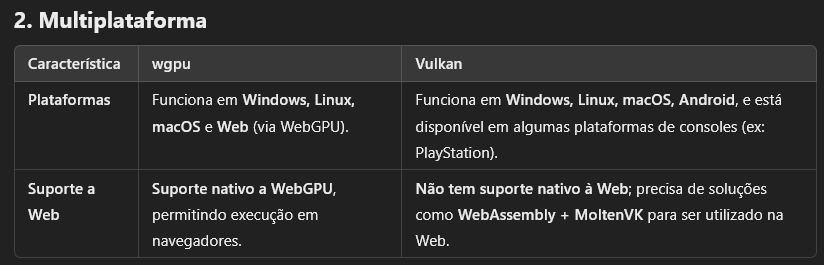
Windows, Linux, Android.
-
No native support for Web, needs WebAssembly.
-
-
Backend:
-
Vulkan
-
-
Focus:
-
High-performance games, advanced 3D graphics
-
-
Advantages:
-
Cross-platform (Windows, Linux, Android)
-
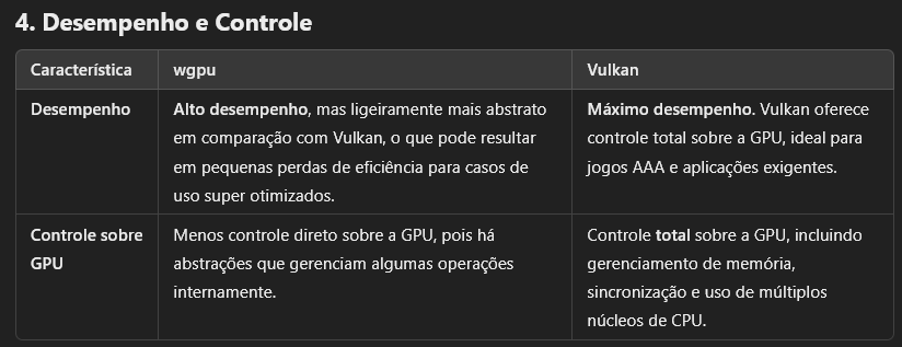
Better performance than OpenGL due to control over the GPU
-
Better management of multiple threads and parallel rendering
-
-
Disadvantages:
-
Complex and difficult to program (similar to DX12).
-
Requires more code and manual memory management
-
More recent support on some platforms (e.g., on macOS, only via layers like MoltenVK)
-
WebGPU
-
WebGPU is an open standard created by the W3C to offer GPU-accelerated graphics and computation within browsers.
-
It is designed to replace WebGL, offering a more modern and efficient API based on Vulkan, Metal, and DirectX 12.
-
Currently, it is being implemented natively in Chrome, Edge, and Firefox.
-
Platforms :
-
Web.
-
Only in browsers compatible with WebGPU.
-
It is not an independent library, but a standard that browsers implement.
-
-
-
Who maintains it :
-
The W3C, in collaboration with major companies like Google, Mozilla, Microsoft, and Apple.
-
-
wgpu :
-
Open-source MIT.
-
It is a native implementation of the WebGPU standard, designed to work both in the browser and in desktop applications.
-
It serves as a cross-platform wrapper that can use different graphics APIs depending on the operating system.
-
Therefore, although WebGPU is a standard for the Web, wgpu is an implementation of that standard that can also run natively outside of browsers.
-
Written in Rust, C/C++, etc.
-
Type:
-
Mid-level graphics API
-
-
Platforms:
-
Windows, Linux, macOS.
-
Web, via WebGPU.
-
-
Supported Backends:
-
Vulkan, DX12, Metal, OpenGL (selected automatically)
-
-
Focus:
-
Cross-platform, WebGPU, ease of use (Rust, C/C++)
-
-
Advantages:
-
Cross-platform and compatible with WebGPU
-
Easier to use than Vulkan/DX12
-
Memory safety and stability
-
-
Disadvantages:
-
Less control over GPU optimizations
-
Still in development, fewer tools than Vulkan/DX12
-
-
-
wgpu vs WebGPU :
-
If you are developing for the Web, you will use WebGPU directly.
-
If you want to use WebGPU also in native apps, wgpu is the right choice, as it allows running the same code both in the browser and on desktops.
-
-
wgpu vs Vulkan :
-
 .
.
-
 .
.
-
 .
.
-
 .
.
-
 .
.
-
 .
.
-
OpenGL
-
OpenGL .
-
Open Source Open Standard.
-
OpenGL itself has not been officially "deprecated" globally, but it is obsolete in many contexts and being replaced by more modern APIs, such as Vulkan.
-
ES 3.x versions are still used on mobile, but Vulkan is the future.
-
-
Type:
-
Mid-level graphics API
-
-
Platforms:
-
Windows, Linux, macOS.
-
Support for Web via WebGL.
-
-
Backend:
-
OpenGL
-
-
Focus:
-
3D graphics for games, graphics engines, scientific applications
-
-
Advantages:
-
Cross-platform and widely supported
-
Easy to use compared to DX12/Vulkan
-
Good documentation and strong community
-
-
Disadvantages:
-
Old API, not optimized for modern GPUs
-
Less control over memory and graphics pipeline
-
Limited support on macOS (Apple uses Metal)
-
WebGL
-
Open Source Open Standard.
-
It is based on OpenGL ES 2.0, which is a simplified version of OpenGL for mobile and embedded devices.
-
WebGPU is the official successor to WebGL.
-
WebGL is still functional, but it is not recommended for new projects.
-
(2025-03-09) There is no official date for removal from browsers.
-
Type:
-
High-level graphics API
-
-
Platforms:
-
Web
-
-
Backend:
-
Based on OpenGL ES 2.0
-
-
Focus:
-
3D rendering on the web
-
-
Advantages:
-
Works directly in the browser, without the need for plugins
-
Easy to learn and integrate into web applications
-
Wide support, compatible with almost all browsers
-
-
Disadvantages:
-
Based on OpenGL ES 2.0, older and less efficient technology
-
No native support for modern features like Ray Tracing and Compute Shaders
-
May have lower performance than WebGPU
-
DirectX 12
-
Closed-source, from Microsoft.
-
Type:
-
Low-level graphics API.
-
-
Platforms:
-
Windows and Xbox
-
-
Backend:
-
Direct3D 12
-
-
Focus:
-
AAA games, high-performance applications
-
-
Advantages:
-
Direct control over the GPU
-
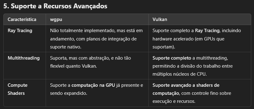
Support for Ray Tracing via DXR
-
Advanced Microsoft tools (PIX, RenderDoc)
-
-
Disadvantages:
-
Only for Windows and Xbox
-
High complexity, requires manual memory management and synchronization.
-
Metal
-
Closed-source, from Apple.
-
Low level and high performance :
-
Reduces CPU overhead, allowing better use of the GPU.
-
-
Support for parallel computation :
-
Includes an API for general computation on the GPU (similar to CUDA or OpenCL).
-
-
Platforms :
-
Exclusive to the Apple ecosystem.
-
Apple discontinued official support for OpenGL and encourages the use of Metal.
-
-
-
Support for Ray Tracing (since Metal 3).
Shader Languages
SPIR-V
GLSL (OpenGL Shader Language)
-
GLSL .
Slang
-
Slang .
WGSL (WebGPU)
-
Modern, safe, and cross-platform (WebGPU standard).
-
Works in browsers (WebGPU) and native (via
wgpu). -
No corporate lock-in (developed by W3C & Mozilla/Google/Apple).
-
Newer, less mature than GLSL/SPIR-V.
-
"Explicitly designed to avoid C++/OOP cruft. Rust-inspired syntax but purely for GPU work."
~HLSL (High-level Shader Language)
-
HLSL .
-
Proprietary to Microsoft.
-
Made for DirectX 9.
-
HLSL programs come in six forms: pixel shaders (fragment in GLSL), vertex shaders, geometry shaders, compute shaders, tessellation shaders (Hull and Domain shaders), and ray tracing shaders.
-
Where it can be used :
-
Is mainly used in DirectX-based environments (Windows/Xbox games, Unity, Unreal Engine). If you're targeting other platforms (macOS, Linux, mobile), you might need to use GLSL, MSL, or SPIR-V instead.
-
Direct3D (DirectX)
-
DirectX 9/10/11/12: HLSL is the standard shading language for Microsoft's Direct3D API.
-
Used in:
-
PC games (Windows)
-
Xbox console development (Xbox One, Xbox Series XS)
-
-
-
Unity (via Direct3D)
-
Unity supports HLSL when using:
-
Built-in Render Pipeline (Legacy)
-
Universal Render Pipeline (URP)
-
High Definition Render Pipeline (HDRP)
-
-
Shader Graph in Unity also uses HLSL-like syntax.
-
-
Unreal Engine (UE4/UE5)
-
Unreal Engine uses a custom shading language (Unreal Shader System, USS) but allows HLSL snippets in Custom HLSL Nodes.
-
HLSL is also used in Ray Tracing shaders in UE5.
-
-
NVIDIA OptiX (Ray Tracing)
-
HLSL can sometimes be used alongside CUDA/PTX for ray tracing effects.
-
-
Vulkan (via SPIR-V Cross)
-
HLSL shaders can be converted to SPIR-V (Vulkan's intermediate format) using tools like:
-
glslangValidator (from Khronos)
-
DXC (DirectX Shader Compiler)
-
SPIRV-Cross (converts HLSL to GLSL/SPIR-V)
-
-
-
Shader Model 6.0+ (Advanced Features)
-
HLSL supports modern GPU features like:
-
Ray Tracing (DXR)
-
Mesh & Amplification Shaders
-
Wave Operations.
-
-
-
Compute Shaders
-
(GPGPU programming in DirectX).
-
-
AI/ML Acceleration
-
(Some frameworks allow HLSL-based compute shaders for GPU acceleration).
-
-
-
Where it's not used :
-
OpenGL / WebGL → Uses GLSL instead.
-
Vulkan (Native) → Uses GLSL or SPIR-V.
-
Metal (Apple) → Uses MSL (Metal Shading Language).
-
-
Ex :
// Vertex Shader struct VSInput { float3 position : POSITION; float3 color : COLOR; }; struct VSOutput { float4 position : SV_POSITION; float3 color : COLOR; }; VSOutput VS_main(VSInput input) { VSOutput output; output.position = float4(input.position, 1.0); output.color = input.color; return output; } // Fragment Shader struct PSInput { float4 position : SV_POSITION; float3 color : COLOR; }; float4 PS_main(PSInput input) : SV_TARGET { return float4(input.color, 1.0); } -
Comparing the syntax of HLSL to GLSL :
-
Inputs :
-
HLSL:
-
The parameter for the
VS_mainandPS_maindescribe the inputs for each step. -
Uses a struct with semantics (
: POSITION,: COLOR).
-
-
GLSL:
-
Uses
in/outvariables. -
Uses
layout(location)to bind vertex attributes.
-
-
-
Outputs :
-
HLSL:
Returns a struct, for passing values from the Vertex Shader to the Fragment Shader;VSOutput. -
GLSL:
-
Uses a
outvariable.
-
-
-
MSL (Metal Shading Language)
-
Apple’s official shader language (optimized for M1/M2).
-
Required for iOS/macOS Metal apps.
-
Apple-only (no Windows/Linux).
-
Use with MoltenVK if you want Vulkan → Metal compatibility.
-
Ex :
// Vertex Shader
#include <metal_stdlib>
using namespace metal;

struct VertexIn {
    float3 position [[attribute(0)]];
    float3 color [[attribute(1)]];
};

struct VertexOut {
    float4 position [[position.md]];
    float3 color;
};

vertex VertexOut vertex_main(VertexIn in [[stage_in]]) {
    VertexOut out;
    out.position = float4(in.position, 1.0);
    out.color = in.color;
    return out;
}

// Fragment Shader
fragment float4 fragment_main(VertexOut in [[stage_in]]) {
    return float4(in.color, 1.0);
}
Tools
Capture
GFXReconstruct
-
Captures commands to a file and allows you to replay them.
-
Linux, Android, Linux.
-
Vulkan, but also other APIs.
-
(2025-10-04)
-
I tested it and it worked nicely, super simple.
-
set VK_INSTANCE_LAYERS=VK_LAYER_LUNARG_gfxreconstruct
set GFXRECON_CAPTURE_FILE=C:\captures\capture.gfxr
set GFXRECON_CAPTURE_FRAMES=1000-2200
my_game.exe
-
gfxrecon-replay-
Tool to replay GFXReconstruct capture files.
gfxrecon-replay --pause-frame 1200 capture.gfxr-
Also supports
--screenshotsand--screenshot-allif you want a quick visual scan of frames. -
While
gfxrecon-replayis paused, attach RenderDoc or Nsight Graphics to the replay process (or launch the replay from RenderDoc/Nsight) and use RenderDoc’s per-draw inspection / pixel history / depth buffer views. The GFXReconstruct docs explicitly say capture files “can be replayed inside other tools (RenderDoc, Nsight, AMD tools, etc.)”.
-
-
gfxrecon-info-
Tool to print information describing GFXReconstruct capture files.
-
-
gfxrecon-compress-
Tool to compress/decompress GFXReconstruct capture files.
-
The gfxrecon-compress tool requires LZ4, Zstandard, and/or zlib, which are currently optional build dependencies.
-
-
gfxrecon-extract-
Tool to extract SPIR-V binaries from GFXReconstruct capture files.
-
-
gfxrecon-convert-
Tool to convert GFXReconstruct capture files to a JSON Lines listing of API calls. (experimental for D3D12 captures)
-
-
gfxrecon-optimize-
Tool to produce new capture files with improved replay performance.
-
Debuggers
RenderDoc
-
-
API loader.
-
-
Cross-platform.
-
Open-source.
-
Not a profiler.
-
RenderDoc is not designed as a continuous multi-second timeline tracer; its strength is detailed single-frame analysis.
Nvidia Nsight Graphics
-
Capture :
-
(2025-10-04)
-
Exceptionally similar to RenderDoc.
-
-
-
GPU Trace :
PIX
-
.
Profilers
Choosing the Space to compute Lighting
-
For more information about precision, check Graphics and Shaders#Precision .
View Space
-
Advantages :
-
Since view space places the camera at the origin, numbers tend to stay small and preserve precision. This is an important consideration when rendering large worlds. When coordinates become large (e.g. 1000km, they cannot represent small differences; details smaller than ~6 cm are lost.
-
View-space normals allow efficient compression: since the camera always looks down the −Z axis, we only need to store x and y components and reconstruct z, saving G-buffer bandwidth. This is a reason why several engines prefer view-space normals for deferred shading. With smaller positions, depth reconstruction is also more stable. This compression does not work for world-space normals, where all directions are equally likely.
-
The view vector in specular/PBR models is simply the negative fragment position in view space. The camera position is (0,0,0), so no extra subtraction is needed. LearnOpenGL notes that this makes the specular term easy to compute and is why many tutorials prefer view-space lighting.
-
LearnOpenGL:
-
We chose to do the lighting calculations in world space, but most people tend to prefer doing lighting in view space.
-
An advantage of view space is that the viewer's position is always at
(0,0,0)so you already got the position of the viewer for free. -
However, I find calculating lighting in world space more intuitive for learning purposes.
-
-
-
Since the fragment’s z value directly represents the distance from the camera, effects like fog, attenuation and cluster slicing in clustered shading become easier to implement.
-
-
Disadvantages :
-
Environment maps and image-based lighting (IBL) are usually defined in world space. To sample them, view-space normals must be converted to world space; repeated conversions can add instructions and risk precision loss. Some encoding techniques only support world-space normals.
-
Because view-space normals rotate with the camera, specular highlights and reflections may appear to wobble, especially when using normal maps.
-
Light positions and directions stored in world space must be transformed into view space each frame. For many lights, this transformation may be non-negligible (though compute shaders can handle it efficiently).
-
World Space
-
Advantages :
-
World-space normals do not change when the camera moves, so specular highlights from normal maps remain stable. This is useful for physically based rendering (PBR) with image-based lighting, where a consistent normal is needed to look up from environment maps.
-
Krzysztof Narkowicz (UE5) notes that world-space normals have beneficial properties: they do not depend on the camera, so specular highlights and reflections on static objects will not wobble when the camera moves. Because their precision does not depend on the camera direction, they remain accurate even for surfaces pointing away from the viewer. In contrast, view-space normals change orientation when the camera rotates, which can make environment map lookups or specular highlights less stable.
-
Since most lights and environment maps are defined in world space, you avoid per-fragment transformations. In forward renderers this can simplify the shader because light direction can be computed once in world space and reused.
-
Some post-processing effects (SSAO, screen-space reflections) and global illumination techniques operate in world space and expect world-space positions and normals. Having them already in world space can avoid conversions.
-
-
Disadvantages :
-
Using world-space positions directly means adding large translations (e.g., the camera is at 1 km while shading a small object). The article “The Perils of World Space” explains that 32-bit floats only have high resolution near the origin; far from the origin, sub-centimetre differences cannot be represented. Thus shading calculations (e.g., diffuse or specular dot products) may wobble due to imprecision. This can manifest as flickering when the camera moves.
-
World-space normals require all three components to be stored, and world-space positions might need 3×32-bit floats. This increases memory bandwidth in deferred renderers compared with view-space normals, which can be compressed.
-
For specular reflections relative to the camera, you must compute the view vector by subtracting the camera position from the fragment position, adding per-fragment cost.
-
-
Trick to improve precision: Fixing the camera and moving the world :
-
Instead of letting the camera roam far from the origin, move the world in the opposite direction so that the camera stays near the origin. Pharr describes decomposing the view matrix into rotation and translation, then moving the translation into the model matrices while keeping the camera at the origin;
worldPos – cameraPosis computed in double-precision on the CPU and passed to the GPU as a small value. Many engines (e.g., Cryengine) perform lighting in world space but shift the origin per frame; this provides the stability of view-space lighting while retaining the advantages of world-space normals
-
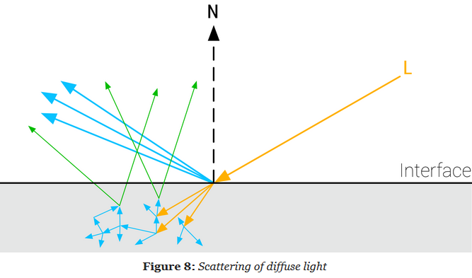
BSDF (Bidirectional Scattering Distribution Function)
Sources
-
-
"Filament pbr paper is nice and readable and even has some pseudo code examples. the renderer is open source (which is also a good reference)".
-
"it just cuts right through the BS and just gives you the math you need".
-
-
Moving Frostbite to Physically Based Rendering 3.0 - Siggraph 2014 .
-
PBR Book.-
Award academy winning book.
-
Basically created the meaning of PBR.
-
"I'm finding myself pretty annoyed at how OOP-y it is so far (I think I'm at 4 levels of inheritancs now for the integrators?)".
-
-
(2025-09-10)
-
The reading sounds sloooow and seems to have the CMake mentality.
-
Nah fok off.
-
-
-
-
It's a super short and not enlightening explanation. The Filament PBR is better.
-
Samples
-
-
"wrap lighting" →
max((dot(N,L) + wrap) / (1+wrap), 0)creates softer shading. -
Can quantize light intensity into bands for toon-like shading.
-
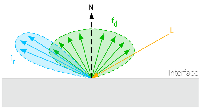
Rendering Equation
BSDF (Bidirectional Scattering Distribution Function)
-
A material model is described mathematically by a BSDF (Bidirectional Scattering Distribution Function), which is itself composed of two other functions:
-
BRDF (Bidirectional Reflectance Distribution Function)
-
BTDF (Bidirectional Transmittance Function).
-
-
Since we aim to model commonly encountered surfaces, our standard material model will focus on the BRDF and ignore the BTDF, or approximate it greatly.
-
-
{9:57}
-
Implementation.
-
-
-
Rendering Equation and BRDFs .
-
Great video, super important to understand rendering and Physics Based Rendering (PBR).
-
Everything is based on the abstract equation, as being the basis for Based Physics Rendering:
-
outgoing_light = emitted_light + reflected_light.
-
-
{10:19}
-
The 'reflected_light' equation is shown
-
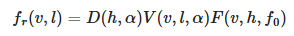
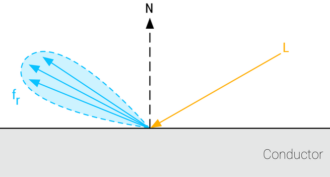
$f_r(x, \omega_i, \omega_o)$ is the 'Bidirectional Reflectance Distribution Function (BRDF)'
-
$L_i$ is the 'color of light'.
-
$cos(\theta_i)$ is the representation of the 'Surface Normal'
-
~Then an integral is used to calculate this at different angles, ~I don't know.
-
Engines don't use the integral.
-
-
-
{10:53}
-
Rendering Equation.
-
-
{22:58 -> end}
-
It's the most interesting part of the video, although everything is interesting.
-
Each parameter of the shader used by Disney is explained.
-
-
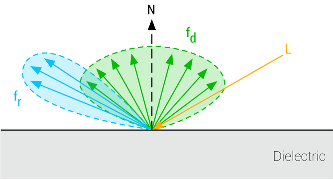
BRDF (Bidirectional Reflectance Distribution Function)
-
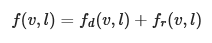
The BRDF describes the surface response of a standard material as a function made of two terms:
-
A diffuse component ($f_d$).
-
A specular component ($f_r$).
-
-
 .
.
-
The complete surface response can be expressed as such:
-
 .
.
-
This equation characterizes the surface response for incident light from a single direction. The full rendering equation would require to integrate $l$ over the entire hemisphere.
-
Energy conservation is one of the key components of a good BRDF for physically based rendering. An energy conservative BRDF states that the total amount of specular and diffuse reflectance energy is less than the total amount of incident energy. Without an energy conservative BRDF, artists must manually ensure that the light reflected off a surface is never more intense than the incident light.
General Terms
-
$v$
-
View unit vector.
-
-
$h$
-
Half unit vector between $l$ and $v$.
-
-
$l$
-
Incident light unit vector.
-
-
$n$
-
Normal surface unit vector.
-
-
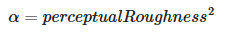
$\alpha$
-
Roughness, remapped from using input
perceptualRoughness.
-
TLDR
-
Specular Term :
-
A Cook-Torrance specular microfacet model
-
A GGX normal distribution function
-
A Smith-GGX height-correlated visibility function.
-
A Schlick Fresnel function.
-
-
Diffuse Term :
-
A Lambertian diffuse model.
-
float D_GGX(float NoH, float a) {
    float a2 = a * a;
    float f = (NoH * a2 - NoH) * NoH + 1.0;
    return a2 / (PI * f * f);
}

vec3 F_Schlick(float u, vec3 f0) {
    return f0 + (vec3(1.0) - f0) * pow(1.0 - u, 5.0);
}

float V_SmithGGXCorrelated(float NoV, float NoL, float a) {
    float a2 = a * a;
    float GGXL = NoV * sqrt((-NoL * a2 + NoL) * NoL + a2);
    float GGXV = NoL * sqrt((-NoV * a2 + NoV) * NoV + a2);
    return 0.5 / (GGXV + GGXL);
}

float Fd_Lambert() {
    return 1.0 / PI;
}

void BRDF(...) {
    // >> Standard Model

    vec3 h = normalize(v + l);

    float NoV = abs(dot(n, v)) + 1e-5;
    float NoL = clamp(dot(n, l), 0.0, 1.0);
    float NoH = clamp(dot(n, h), 0.0, 1.0);
    float LoH = clamp(dot(l, h), 0.0, 1.0);

    // perceptually linear roughness to roughness (see parameterization)
    float roughness = perceptualRoughness * perceptualRoughness;

    float D = D_GGX(NoH, roughness);
    vec3  F = F_Schlick(LoH, f0);
    float V = V_SmithGGXCorrelated(NoV, NoL, roughness);

    // specular BRDF
    float D = distributionCloth(roughness, NoH);  // From the Cloth BRDF.
    float V = visibilityCloth(NoV, NoL);          // From the Cloth BRDF.
    vec3  F = sheenColor;                         // From the Cloth BRDF.
    vec3 Fr = (D * V) * F;

    vec3 energyCompensation = 1.0 + f0 * (1.0 / dfg.y - 1.0);
    // Scale the specular lobe to account for multiscattering
    Fr *= pixel.energyCompensation;

    // Without Cloth BRDF
    // diffuse BRDF
    // Conversion of base color to diffuse:
    vec3 diffuseColor = (1.0 - metallic) * baseColor.rgb;
    vec3 Fd = diffuseColor * Fd_Lambert();

    // With Cloth BRDF
    float diffuse = diffuse(roughness, NoV, NoL, LoH);
    #if defined(MATERIAL_HAS_SUBSURFACE_COLOR)
    // energy conservative wrap diffuse
    diffuse *= saturate((dot(n, light.l) + 0.5) / 2.25);
    #endif
    vec3 Fd = diffuse * pixel.diffuseColor;

    // <<


    // >> Cloth BRDF

    #if defined(MATERIAL_HAS_SUBSURFACE_COLOR)
    // cheap subsurface scatter
    Fd *= saturate(subsurfaceColor + NoL);
    vec3 color = Fd + Fr * NoL;
    color *= (lightIntensity * lightAttenuation) * lightColor;
    #else
    vec3 color = Fd + Fr;
    color *= (lightIntensity * lightAttenuation * NoL) * lightColor;
    #endif

    // <<


    // >> Clear Coat

    // remapping and linearization of clear coat roughness
    clearCoatPerceptualRoughness = clamp(clearCoatPerceptualRoughness, 0.089, 1.0);
    clearCoatRoughness = clearCoatPerceptualRoughness * clearCoatPerceptualRoughness;

    // clear coat BRDF
    float  Dc = D_GGX(clearCoatRoughness, NoH);
    float  Vc = V_Kelemen(clearCoatRoughness, LoH);
    float  Fc = F_Schlick(0.04, LoH) * clearCoat; // clear coat strength
    float Frc = (Dc * Vc) * Fc;

    // <<


    // account for energy loss in the base layer
    return color * ((Fd + Fr * (1.0 - Fc)) * (1.0 - Fc) + Frc);
}


void main() {
    // I believe this is completely geared towards Directional Lights.

    vec3 l = normalize(-lightDirection);
    float NoL = clamp(dot(n, l), 0.0, 1.0);

    // lightIntensity is the illuminance
    // at perpendicular incidence in lux
    float illuminance = lightIntensity * NoL;
    vec3 luminance = BSDF(v, l) * illuminance;
}
Specular BRDF
-
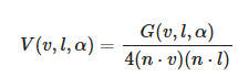
For the specular term, $f_r$ is a mirror BRDF that can be modeled with the Fresnel law , noted in the Cook-Torrance approximation of the microfacet model integration:
-
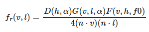 .
.
-
This function can be simplified by introducing a Visibility Function.
-
 .
.
-
 .
.
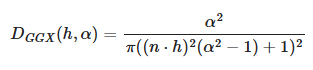
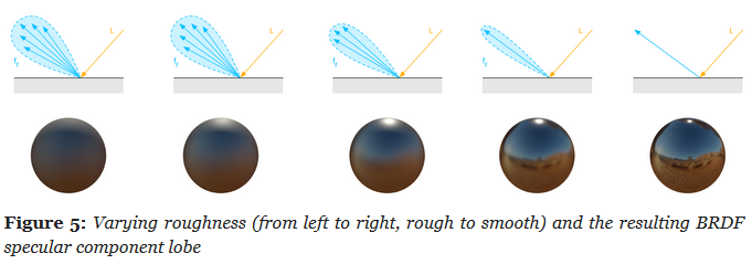
Normal distribution function (Specular D)
-
Burley observed that long-tailed normal distribution functions (NDF) are a good fit for real-world surfaces.
-
The GGX distribution is a distribution with long-tailed falloff and short peak in the highlights, with a simple formulation suitable for real-time implementations. It is also a popular model, equivalent to the Trowbridge-Reitz distribution, in modern physically based renderers.
-
 .
.
-
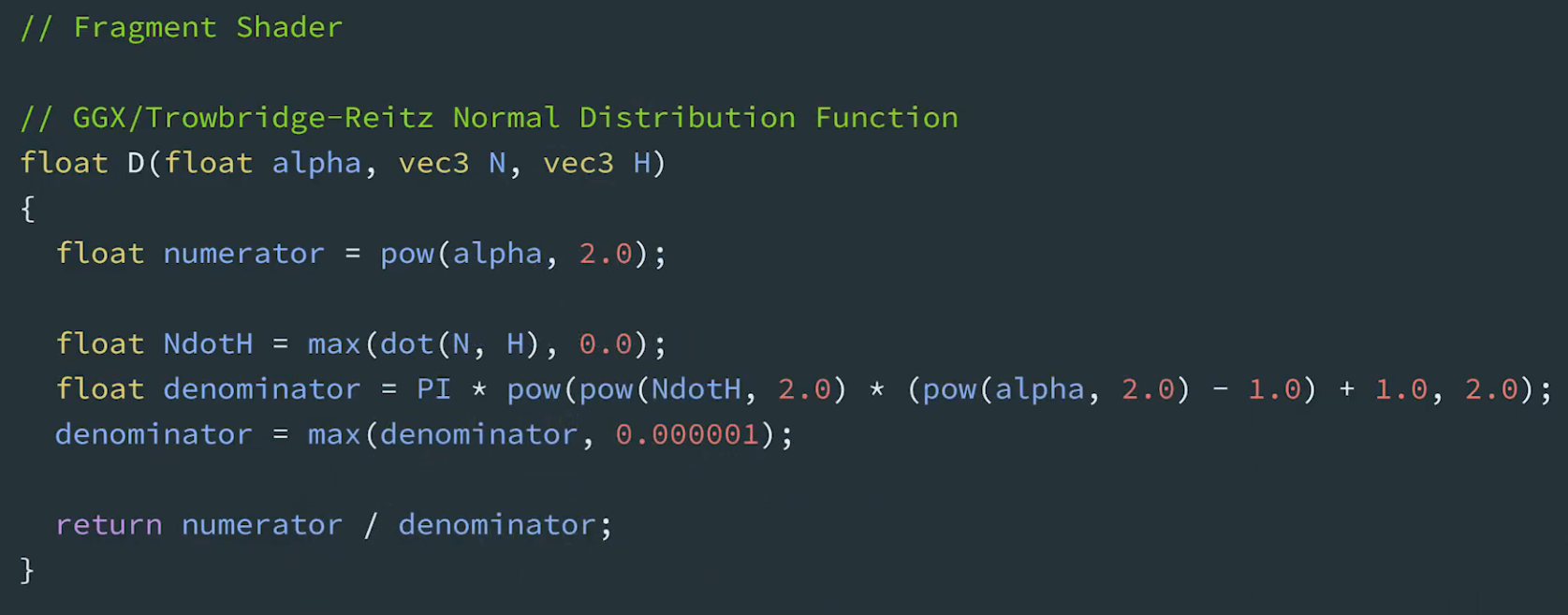
Specular D term :
float D_GGX(float NoH, float roughness) { float a = NoH * roughness; float k = roughness / (1.0 - NoH * NoH + a * a); return k * k * (1.0 / PI); } -
Specular D term, optimized for fp16 :
#define MEDIUMP_FLT_MAX 65504.0 #define saturateMediump(x) min(x, MEDIUMP_FLT_MAX) float D_GGX(float roughness, float NoH, const vec3 n, const vec3 h) { vec3 NxH = cross(n, h); float a = NoH * roughness; float k = roughness / (dot(NxH, NxH) + a * a); float d = k * k * (1.0 / PI); return saturateMediump(d); } -
 .
.
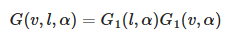
Geometric Shadowing / Visibility Function (Specular G / Specular V)
-
Eric Heitz showed in that the Smith geometric shadowing function is the correct and exact term to use.
-
The Smith formulation is the following:
-
 .
.
-
Consider:
-
Specular V term :
-
The GLSL implementation of the visibility term, is a bit more expensive than we would like since it requires two
sqrtoperations.
float V_SmithGGXCorrelated(float NoV, float NoL, float roughness) { float a2 = roughness * roughness; float GGXV = NoL * sqrt(NoV * NoV * (1.0 - a2) + a2); float GGXL = NoV * sqrt(NoL * NoL * (1.0 - a2) + a2); return 0.5 / (GGXV + GGXL); } -
-
Approximated specular V term :
-
This approximation is mathematically wrong but saves two square root operations and is good enough for real-time mobile applications
float V_SmithGGXCorrelatedFast(float NoV, float NoL, float roughness) { float a = roughness; float GGXV = NoL * (NoV * (1.0 - a) + a); float GGXL = NoV * (NoL * (1.0 - a) + a); return 0.5 / (GGXV + GGXL); }-
(2025-09-13) Note:
-
If roughness is 0, then the final result is
1 / (4 * NoL * NoV). -
I tested this, it's correct.
-
-
-
 .
.
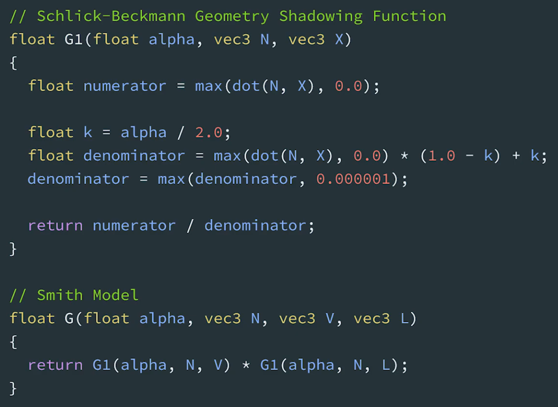
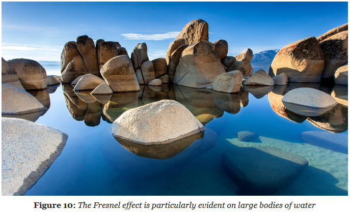
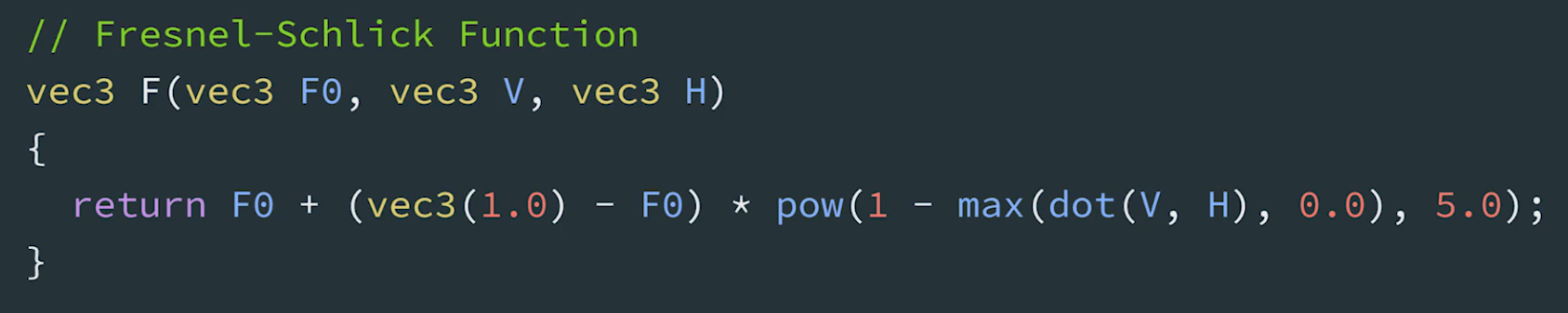
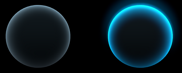
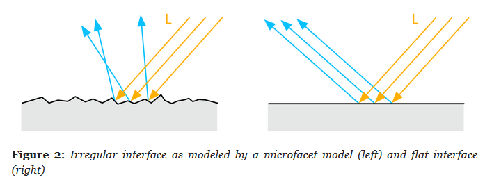
Fresnel (Specular F)
-
This effect models the fact that the amount of light the viewer sees reflected from a surface depends on the viewing angle and on the index of refraction (IOR) of the material.
-
 .
.
-
When looking at the water straight down (at normal incidence) you can see through the water. However, when looking further out in the distance (at grazing angle, where perceived light rays are getting parallel to the surface), you will see the specular reflections on the water become more intense.
-
-
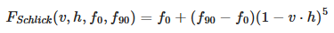
Schlick describes an inexpensive approximation of the Fresnel term for the Cook-Torrance specular BRDF:
-
 .
.
-
This Fresnel function can be seen as interpolating between the incident specular reflectance and the reflectance at grazing angles.
-
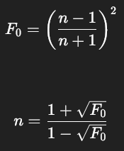
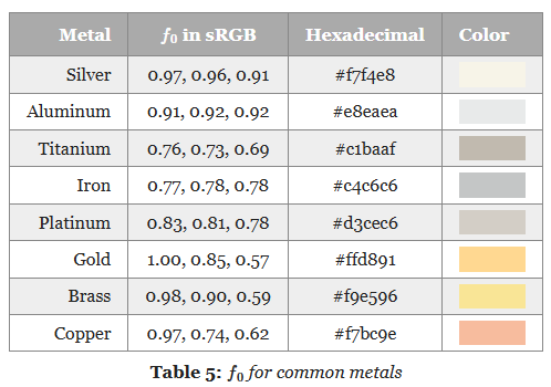
$f_0$ (Base Reflectance or Base Reflectivity) :
-
Is a constant that represents the specular reflectance at normal incidence and is achromatic for dielectrics, and chromatic for metals.
-
The actual value depends on the index of refraction of the interface.
-
If dia-electric: use base reflectivity of 0.04; else: is a metal, use albedo as base reflectivity.
-
n (Index of Refraction) (IOR) :
-
base_reflectivity of 0.04 is the same as IOR = 1.5.
-
IOR 1.5 is the default for blender.
-
 .
.
-
-
Calculating $f_0$ and Remapping :
-
The Fresnel term relies on $f_0$ , the specular reflectance at normal incidence angle, and is achromatic for dielectrics.
-
Remapping :
vec3 f0 = 0.16 * reflectance * reflectance-
See the Material -> Reflectance part to understand the remapping.
-
-
Computing $f_0$ for dielectric and metallic materials in GLSL
vec3 f0 = 0.16 * reflectance * reflectance * (1.0 - metallic) + baseColor * metallic; -
-
-
$f_{90}$.
-
Reflectance at grazing angles.
-
Approaches 100% for smooth materials.
-
Observation of real world materials show that both dielectrics and conductors exhibit achromatic specular reflectance at grazing angles and that the Fresnel reflectance is 1.0 at 90°.
-
-
Specular F term :
vec3 F_Schlick(float u, vec3 f0, float f90) { return f0 + (vec3(f90) - f0) * pow(1.0 - u, 5.0); }-
Using $f_{90}$ set to 1, the Schlick approximation for the Fresnel term can be optimized for scalar operations by refactoring the code slightly.
vec3 F_Schlick(float u, vec3 f0) { float f = pow(1.0 - u, 5.0); return f + f0 * (1.0 - f); }-
 .
.
-
Godot Code Snippet :
float fresnel(float amount, vec3 normal, vec3 view) { return pow((1.0 - clamp(dot(normalize(normal), normalize(view)), 0.0, 1.0 )), amount); } void fragment() { vec3 base_color = vec3(0.0); float basic_fresnel = fresnel(3.0, NORMAL, VIEW); ALBEDO = base_color + basic_fresnel; }-
Colorful Fresnel:
-
This snippet lets you colorize the fresnel by multiplying it with an RGB-value and set the intensity to either tone down the effect or, if you crank it up, make it glow. You need to enable Glow in the Environment node. (The
clamp()has been removed allowing the fresnel to go beyond 1.0). You can also make the fresnel glow by assigning it to EMISSION. -
 .
.
-
Not-colorful / colorful + glow.
-
vec3 fresnel_glow(float amount, float intensity, vec3 color, vec3 normal, vec3 view) { return pow((1.0 - dot(normalize(normal), normalize(view))), amount) * color * intensity; } void fragment() { vec3 base_color = vec3(0.5, 0.2, 0.9); vec3 fresnel_color = vec3(0.0, 0.7, 0.9); vec3 fresnel = fresnel_glow(4.0, 4.5, fresnel_color, NORMAL, VIEW); ALBEDO = base_color + fresnel; } -
-
-
Energy Compensation
-
 .
.
-
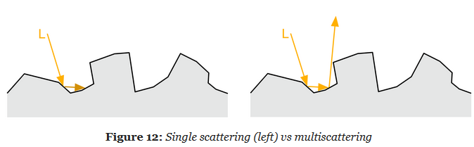
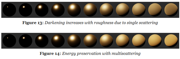
Single Scaterring vs Multiscattering :
-
 .
.
-
 .
.
-
-
This solution is therefore not suitable for real-time rendering.
-
The idea is to add an energy compensation term as an additional BRDF lobe.
vec3 energyCompensation = 1.0 + f0 * (1.0 / dfg.y - 1.0);
// Scale the specular lobe to account for multiscattering
Fr *= pixel.energyCompensation;
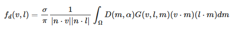
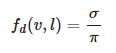
Diffuse BRDF
-
The diffuse term of the BRDF:
-
 .
.
-
Our implementation will instead use a simple Lambertian BRDF that assumes a uniform diffuse response over the microfacets hemisphere:
-
 .
.
-
Diffuse Lambertian BRDF :
-
In practice, the diffuse reflectance is multiplied later
float Fd_Lambert() { return 1.0 / PI; } vec3 Fd = diffuseColor * Fd_Lambert(); -
-
However, the diffuse part would ideally be coherent with the specular term and take into account the surface roughness. Both the Disney diffuse BRDF and Oren-Nayar model take the roughness into account and create some retro-reflection at grazing angles. Given our constraints we decided that the extra runtime cost does not justify the slight increase in quality. This sophisticated diffuse model also renders image-based and spherical harmonics more difficult to express and implement.
-
Disney diffuse BRDF :
-
 .
.
-
 .
.
float F_Schlick(float u, float f0, float f90) { return f0 + (f90 - f0) * pow(1.0 - u, 5.0); } float Fd_Burley(float NoV, float NoL, float LoH, float roughness) { float f90 = 0.5 + 2.0 * roughness * LoH * LoH; float lightScatter = F_Schlick(NoL, 1.0, f90); float viewScatter = F_Schlick(NoV, 1.0, f90); return lightScatter * viewScatter * (1.0 / PI); } -
-
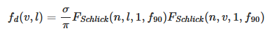
Lambertian diffuse BRDF vs Disney diffuse BRDF :
-
The material used is fully dialetric.
-
The surface response is very similar with both BRDFs but the Disney one exhibits some nice retro-reflections at grazing angles (look closely at the left edge of the spheres).
-
 .
.
-
We could allow artists/developers to choose the Disney diffuse BRDF depending on the quality they desire and the performance of the target device. It is important to note however that the Disney diffuse BRDF is not energy conserving as expressed here.
-
Material
Base Color / Albedo
-
Diffuse albedo for non-metallic surfaces, and specular color for metallic surfaces.
-
Linear RGB
[0..1]. -
It should be devoid of lighting information, except for micro-occlusion.
-
For Non-Metallic Materials :
-
Represents the reflected color and should be an sRGB value in the range 50-240 (strict range) or 30-240 (tolerant range).
-
-
For Metallic Materials :
-
Represents both the specular color and reflectance.
-
Use values with a luminosity of 67% to 100% (170-255 sRGB).
-
Oxidized or dirty metals should use a lower luminosity than clean metals to take into account the non-metallic components.
-
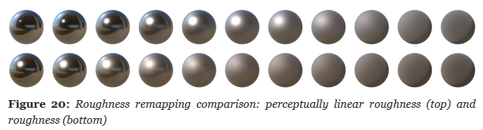
Roughness Value / Roughness Map
-
Perceived smoothness (0.0) or roughness (1.0) of a surface. Smooth surfaces exhibit sharp reflections
-
Scalar
[0..1]. -
 .
.
-
Rough (left), smooth (right).
-
-
 .
.
-
Remapping :
-
 .
.
-
 .
.
-
Metallic Map
-
Whether a surface appears to be dielectric (0.0) or conductor (1.0).
-
Scalar
[0..1]. -
Is almost a binary value. Pure conductors have a metallic value of 1 and pure dielectrics have a metallic value of 0. You should try to use values close at or close to 0 and 1. Intermediate values are meant for transitions between surface types (metal to rust for instance).
-
 .
.
-
Non-Metallic.
-
-
 .
.
-
Metallic.
-
Reflectance
Parameter
-
Fresnel reflectance at normal incidence for dielectric surfaces. This replaces an explicit index of refraction
-
Scalar
[0..1]. -
For Non-Metallic Materials :
-
Should be set to 127 sRGB (0.5 linear, 4% reflectance) if you cannot find a proper value. Do not use values under 90 sRGB (0.35 linear, 2% reflectance).
-
-
For Metallic Materials :
-
Is ignored (calculated from the base color).
-
-
We will use the remapping for dielectric surfaces:
-
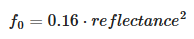 .
.
-
For
reflectance = 0.5,f0 = 0.04.
-
-
The goal is to map onto a range that can represent the Fresnel values of both common dielectric surfaces (4% reflectance) and gemstones (8% to 16%).
-
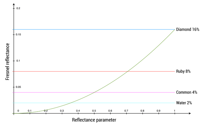 .
.
-
The mapping function is chosen to yield a 4% Fresnel reflectance value for an input reflectance of 0.5 (or 128 on a linear RGB gray scale).
-
 .
.
-
No real world material has a value under 2%.
-
-
 .
.
Emission
-
Additional diffuse albedo to simulate emissive surfaces (such as neons, etc.) This parameter is mostly useful in an HDR pipeline with a bloom pass
-
Linear RGB
[0..1]+ exposure compensation.
Normal Map, Displacement Map
-
Bump, Normal, Displacement, and Parallax Mapping .
-
Great video. No formulas or implementation, though.
-
Displacement Map
-
Actually generate the geometry deformation; it's not faking anything.
-
A lot more expensive then Bump Map or Normal Map.
-
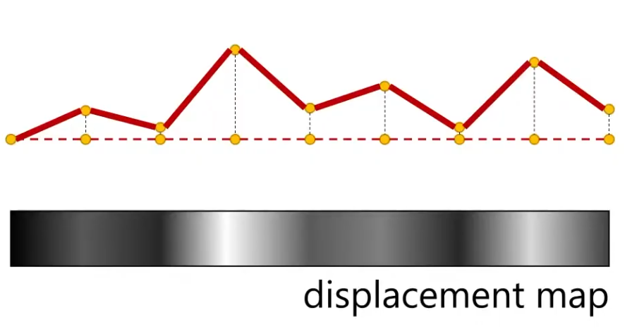 .
.
-
Requirements :
-
You can have a really high-res Displacement Map, but if you don't have enough vertices to displace, then you will not get the geometric detail.
-
This is not the same for Normal Maps; a high-res Normal Map give high detail, regardless of the vertex count.
-
-
-
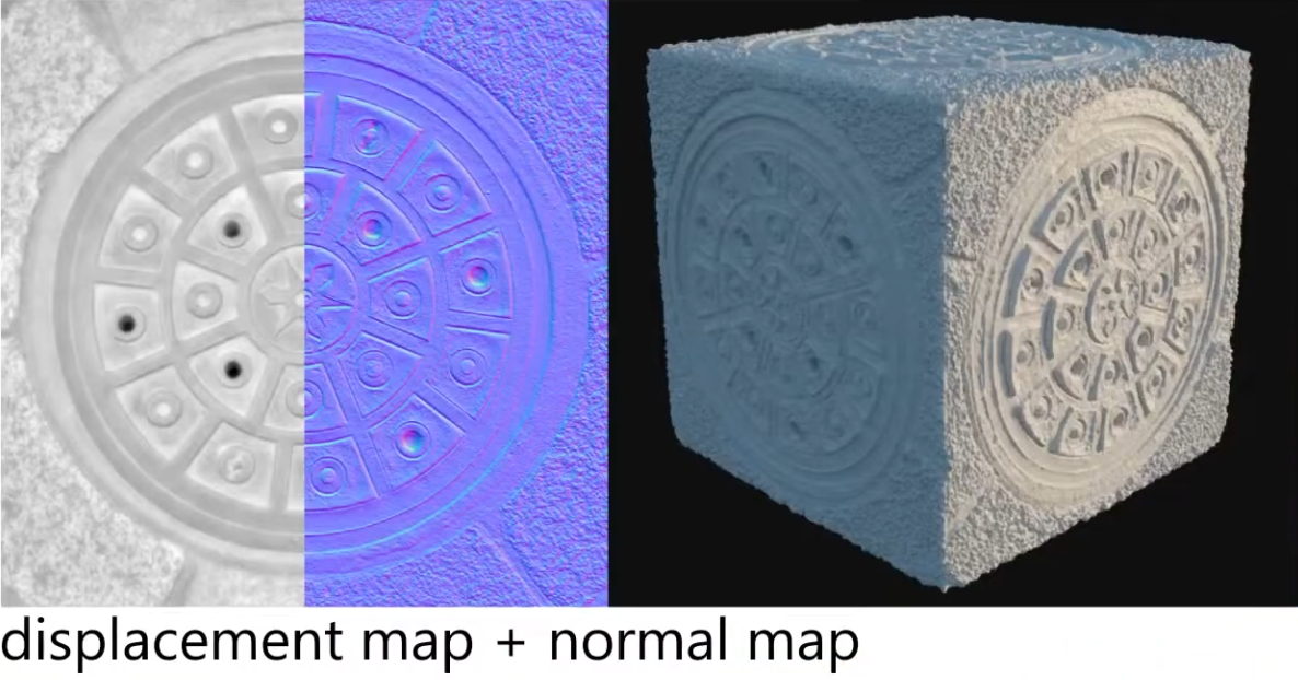
Displacement Map vs Displacement Map + Normal Map
-
The Displacement Map is usually used with a Normal Map.
-
Just by moving vertices around, you are not changing the normals. To see the visual changes, you need the normals that the geometry will have after the displacement.
-
How can I get the Normal Map? You can use the Displacement Map as a Bump Map, which will give you the information you need to get the Normal Map.
-
You should have a Normal Map if you intend to use the Displacement Map at runtime, as it's cheaper then having to calculate the normals on the fly.
-
-
 .
.
-
You can use a Displacement Map without a Normal Map, but you need to "apply" the Displacement Map so you calculate the new normals after the Displacement.
-
If you don't apply (and thus re-calculate the surface normals), you will need a Normal Map.
-
In the end, you need the new normals, in one way or another.
-
-
Used for :
-
Offline Terrain Generation.
-
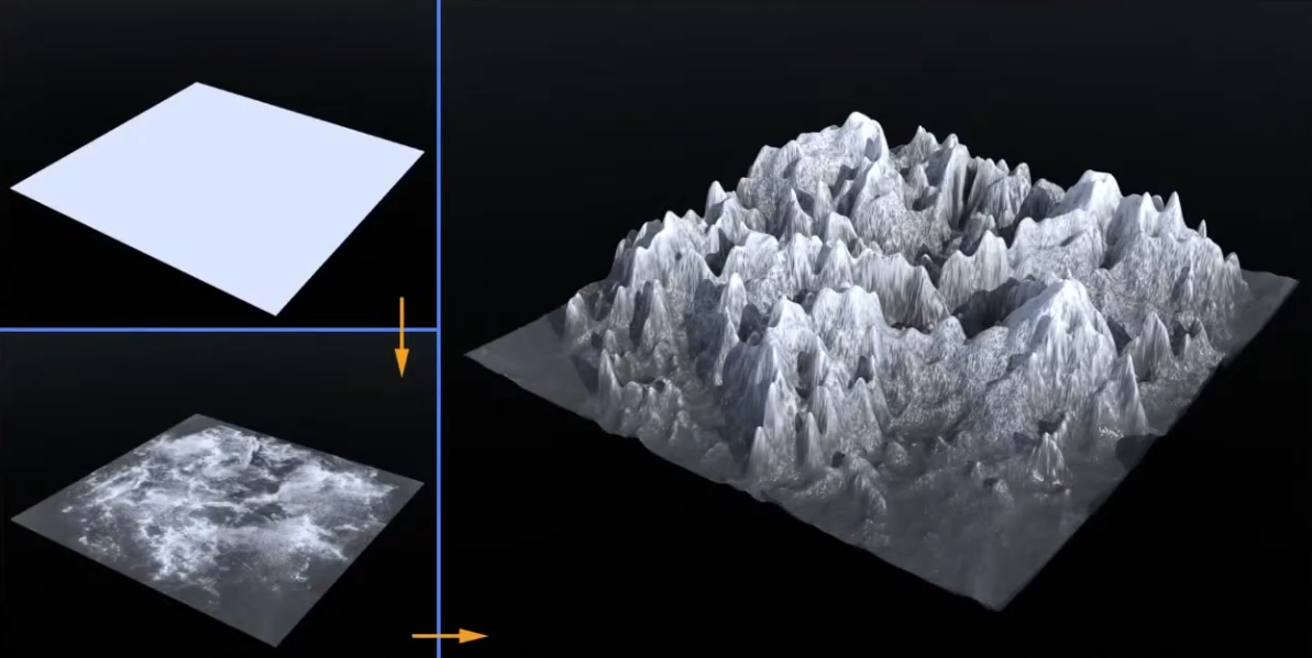 .
.
-
-
Offline Sculptures.
-
Some fine details that are hard to model, and you may want geometry, instead of faking with a Normal Map.
-
 .
.
-
-
-
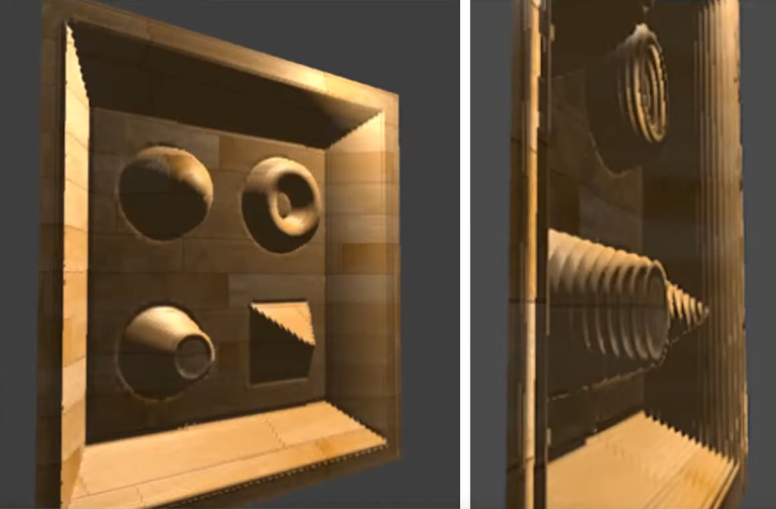
Per-Pixel Displacement Mapping :
-
It's a technique to get the visual of a displacement map, without generating new geometry.
-
The trick is not elevating the geometry with the Displacement Mapping, but "craving" the geometry.
-
 .
.
-
Renders the green point, instead of the blue point.
-
-
This is a lot cheaper then having a Displacement Map generating the geometry, but still has a cost, as the fragment shader needs to figure out what pixel to actually shade.
-
-
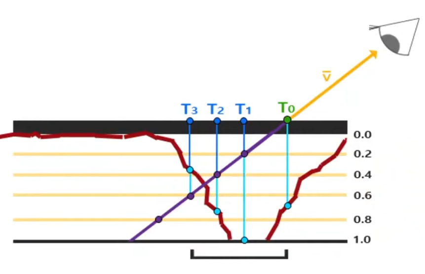
Parallax Mapping :
-
Is a way to approximate the result of Per-Pixel Displacement Mapping .
-
 .
.
-
With Per-Pixel Displacement Mapping , the frag shader would have to figure out what's the correct point to shade. It will look for the blue point B.
-
With Parallax Mapping , the height between the A point and the correct height H(A) is used as an approximation to determine where the blue point B is. In this example, the technique misses the B point and reaches P, but this is the final pixel that will be drawn.
-
Even tho seems like a "big miss", the final visual looks fine.
-
-
-
 .
.
-
 .
.
-
If the surface is rotated, things begin to not look so good.
-
Looking head on is better.
-
-
-
Steep Parallax Mapping :
-
A better approximation for Per-Pixel Displacement Mapping then Parallax Mapping , but a considerable more expensive then Parallax Mapping .
-
 .
.
-
It does multiple texture reads instead of just one, in order to determine a better "stopping point" for the 'correct pixel to shade'.
-
-
 .
.
-
It's better, but if the angle is too exagerated, the problem returns.
-
-
-
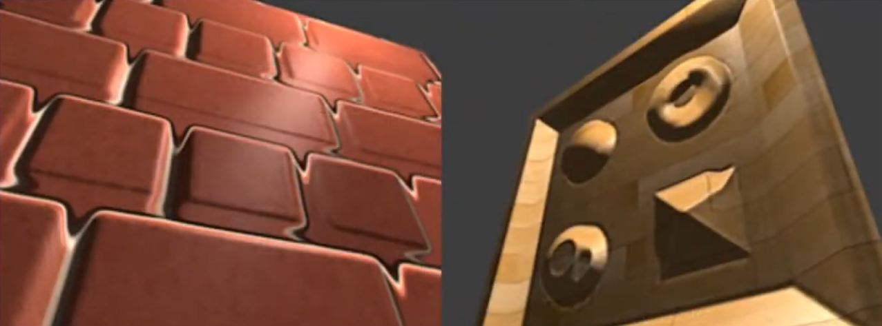
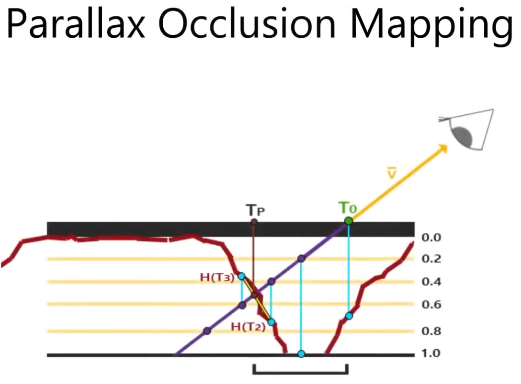
Parallax Occlusion Mapping :
-
A better approximation for Per-Pixel Displacement Mapping then Step Parallax Mapping , but a bit more expensive then Step Parallax Mapping .
-
 .
.
-
It adds one extra step at the end of the Step Parallax Mapping evaluation.
-
This extra step doesn't perform any new texture read, it just better guesses the 'correct pixel to shade' based on the position of the previous step and the final step.
-
-
It gives more "continuity" for the guesses. It's smoother.
-
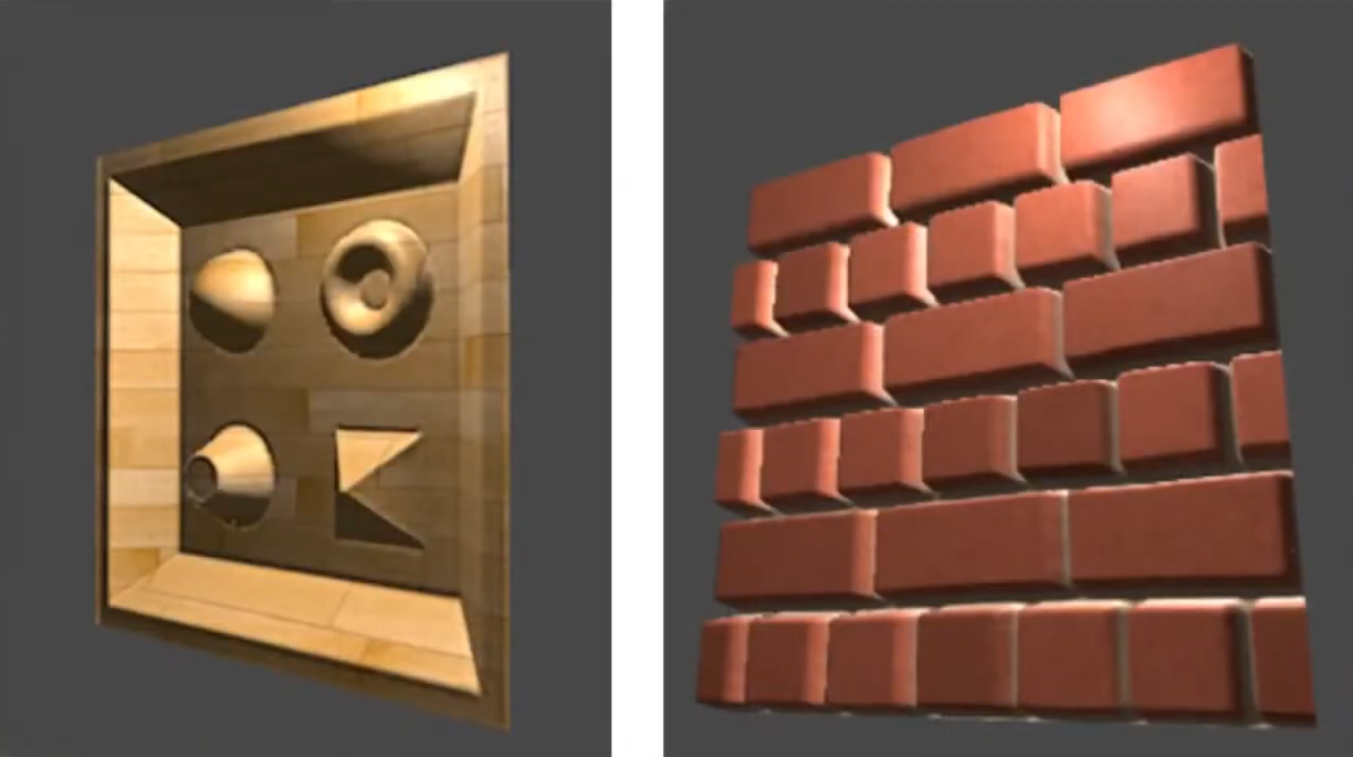 .
.
-
 .
.
-
The stairs uses the Parallax Occlusion Mapping; it's just a flat plain.
-
-
 .
.
-
All the walls uses the Parallax Occlusion Mapping.
-
-
 .
.
-
 .
.
-
-
What about shadow casting?
-
Displacement Mapping and all techniques that approximate the result of Displacement Mapping can cast shadows.
-
 .
.
-
-
WebGL Demo of different displacement techniques .
-
(2025-09-12) Didn't work on Firefox, Brave, or Chrome.
-
Normal Map
-
Tangent Space :
-
Tangent Space - Eric Lengyel .
-
(2025-09-15)
-
This is the one I chose to use.
-
RayLib does this same implementation in
GenMeshTangents.
-
-
-
-
The implementation is designed, specifically, to make the generation of tangent space as resilient as possible to a 3D model being moved from one application to another. That is generate the same tangent spaces even if there is a change in index list(s), ordering of faces/vertices of a face, and/or the removal of degenerate primitives. Both triangles and quads are supported.
-
This makes it easy for anyone to integrate the implementation into their own application and thus reproduce the same tangent spaces. This also makes the code a perfect candidate for an implementation standard. We hope the standard will be adopted by as many developers as possible.
-
The standard is used in Blender 2.57 and is also used by default in xNormal since version 3.17.5 in the form of a built-in tangent space plugin (binary and code).
-
-
-
Example .
-
-
Smooth Shading / Flat Shading :
-
Apparently my procedural Meshes are smooth by default, due to my implementation.
-
If adjacent faces share the same vertex a
-
If triangles do not share vertex normals (i.e., each triangle has its own vertex normal equal to the face normal), lighting will be flat (sharp edges between faces).nd that vertex has a single normal (an average), shading will be smooth across the faces.
-
-
Meshes coming from models may or may not be smooth, depending on how it was imported.
-
-
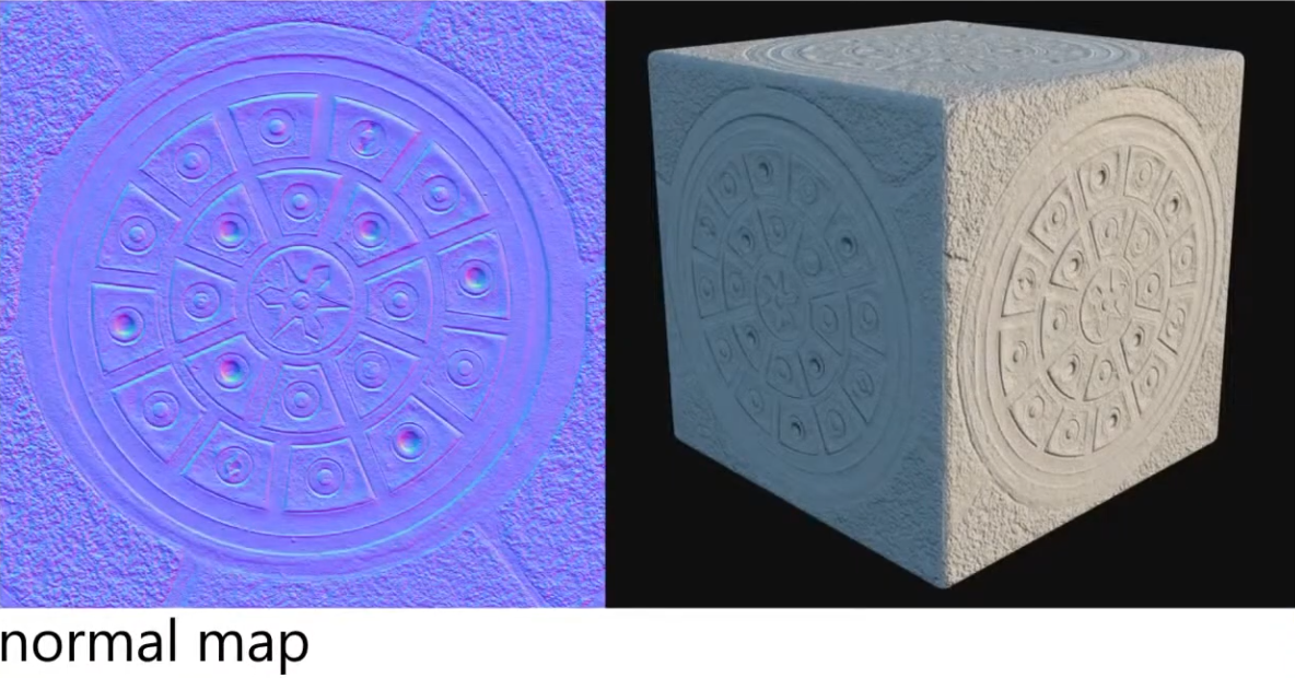
A RGB texture encoding surface normals (X, Y, Z).
-
Overrides per-pixel normal vectors, giving the illusion of complex surface detail under lighting without changing geometry.
-
Used for small details/deformations; doesn't work well for something that is too deep or elevated; the illusion breaks.
-
The coordinates from the Normal Map are actually in local coordinates from the point evaluated.
-
This make sense, as we want the normals to make sense, even if the character is moving.
-
This is why there's a lof of blue in a normal map. The more blue the map is, the less disturbed the normal of a point is.
-
-
Color intuition :
-
Red: inclining the normal towards the X direction (X+ == right).
-
Green: inclining towards the Y direction (Y+ == up).
-
Blue: not inclining.
-
-
 .
.
-
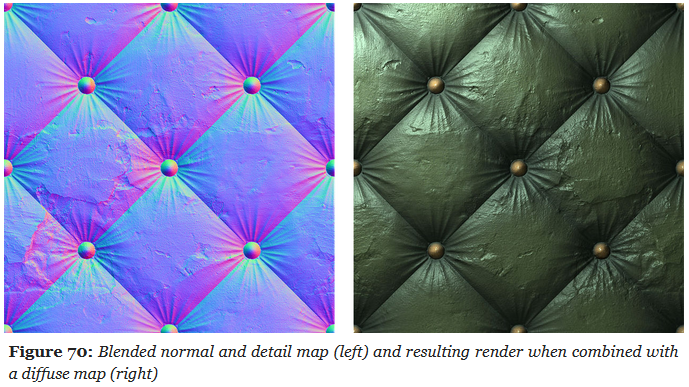
Blending normal maps :
-
Reoriented normal mapping
vec3 t = texture(baseMap, uv).xyz * vec3( 2.0, 2.0, 2.0) + vec3(-1.0, -1.0, 0.0); vec3 u = texture(detailMap, uv).xyz * vec3(-2.0, -2.0, 2.0) + vec3( 1.0, 1.0, -1.0); vec3 r = normalize(t * dot(t, u) - u * t.z); return r;-
 .
.
-
UDN Blending :
-
Its main advantage is the low number of shader instructions it requires.
-
While it leads to a reduction in details over flat areas, UDN blending is interesting if blending must be performed at runtime.
vec3 t = texture(baseMap, uv).xyz * 2.0 - 1.0; vec3 u = texture(detailMap, uv).xyz * 2.0 - 1.0; vec3 r = normalize(t.xy + u.xy, t.z); return r; -
-
~Height Map
-
Usually referred to as a Bump Map, but they aren't really the same.
-
Grayscale texture, encoding relative surface elevation; it represents the actual height/elevation values, not the variations as a Bump Map would do.
-
It can be used in different contexts:
-
To generate normals (essentially turning it into a bump/normal map).
-
To drive parallax mapping (screen-space depth illusion).
-
To drive displacement mapping (real geometric change).
-
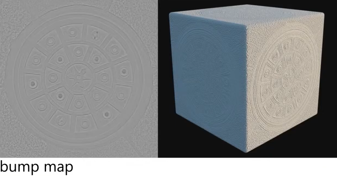
Bump Map
-
Grayscale texture where brightness represents surface height variations . White = high, black = low.
-
It does not store absolute "height," but only brightness variations that are sampled to compute a local slope.
-
No depth, no parallax.
-
Very lightweight (single-channel grayscale).
-
Typically used for adding simple surface detail in older or performance-constrained engines.
-
 .
.
-
Requires additional texture reads. You have to know how the height is changing in regions around the current point.
-
"Would be nice to just pre-record the normals (as that what we actually want), instead of having to compute the normals through a Bump Map? Yes! That's why a Normal Map exists".
-
The Normal Map stores the normals, instead of the variation of the normals, like a Bump Map.
-
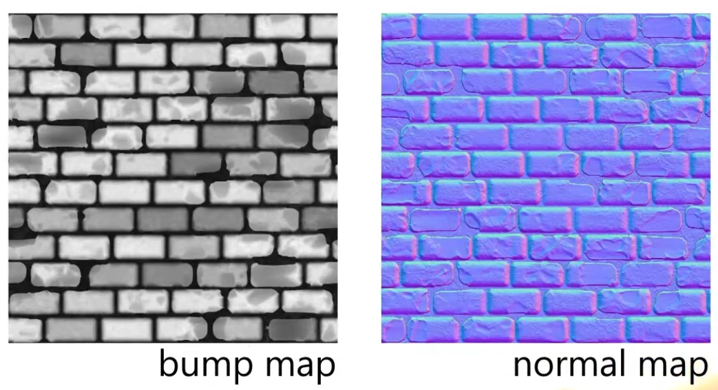 .
.
-
Visually, at runtime, they will look exactly the same; not always, but close enough; the parameters need to be the same.
-
-
Normal Map is the modernized version of a Bump Map.
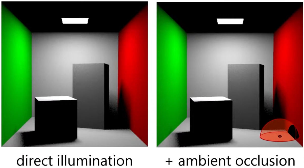
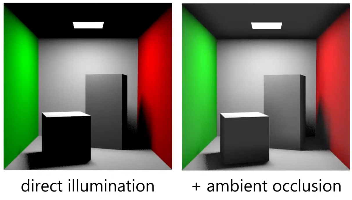
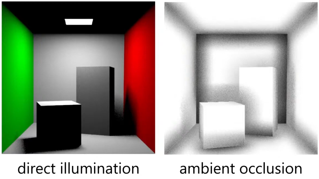
Ambient Occlusion Map
Parameter
-
Defines how much of the ambient light is accessible to a surface point. It is a per-pixel shadowing factor between 0.0 and 1.0.
-
Scalar
[0..1]. -
AO is an approximation of diffuse global illumination , focusing purely on occlusion from nearby geometry, approximating how exposed each point in a scene is to ambient lighting.
-
More specifically, it estimates the amount of indirect light that reaches a surface point by considering occlusion from nearby geometry.
-
Areas that are tightly enclosed or near other surfaces (e.g., corners, creases) receive less ambient light and appear darker.
-
Areas that are more open or exposed receive more ambient light and appear brighter.
-
-
AO is not full global illumination; it ignores directional light transport and color bleeding—it’s a simplified model to capture the general “shadowing” effect of ambient light.
-
The idea for Ambient Occlusion is to determine how bright or dark a region should be based on what is occluding it.
-
 .
.
-
 .
.
-
 .
.
Ambient Occlusion Map
-
Diffuse :
// diffuse indirect vec3 indirectDiffuse = max(irradianceSH(n), 0.0) * Fd_Lambert(); // ambient occlusion indirectDiffuse *= texture2D(aoMap, outUV).r; -
Specular :
float f90 = clamp(dot(f0, 50.0 * 0.33), 0.0, 1.0);
// cheap luminance approximation
float f90 = clamp(50.0 * f0.g, 0.0, 1.0);
float computeSpecularAO(float NoV, float ao, float roughness) { return clamp(pow(NoV + ao, exp2(-16.0 * roughness - 1.0)) - 1.0 + ao, 0.0, 1.0); } // specular indirect vec3 indirectSpecular = evaluateSpecularIBL(r, perceptualRoughness); // ambient occlusion float ao = texture2D(aoMap, outUV).r; indirectSpecular *= computeSpecularAO(NoV, ao, roughness); -
Horizon :
// specular indirect vec3 indirectSpecular = evaluateSpecularIBL(r, perceptualRoughness); // horizon occlusion with falloff, should be computed for direct specular too float horizon = min(1.0 + dot(r, n), 1.0); indirectSpecular *= horizon * horizon; -
Suggestions :
-
TLDR : Option 4 is the correct one, 3 is acceptable in the absence of IBL, and 1 is a non-physics-based hack.
-
~multiply only the albedo.
-
Blender does it this way.
-
I felt that it greatly increases the contrast in the object. Even in the most illuminated points, there are dark regions.
-
If you multiply the base color texture directly by AO (texture-level multiplication), you may inadvertently change the metallic F0 appearance. Avoid multiplying the base color used for F0 in the specular path; instead apply AO only to the diffuse/indirect parts.
-
-
~multiply only the diffuse.
-
I felt that it greatly increases the contrast in the object. Even in the most illuminated points, there are dark regions.
-
Do not multiply light_accumulation by AO — that would darken direct lighting and specular highlights.
-
-
~multiply the ambient_final
-
If you have no IBL yet, multiply the AO into ambient_final. Once you add IBL, multiply AO into the indirect diffuse term (the irradiance / ambient diffuse) and apply a reduced or rougness-weighted AO to the indirect specular if you want occlusion to affect glossy reflections.
-
-
apply only to ambient indirect:
// -> Indirect diffuse (irradiance)
vec3 irradiance; // from diffuse irradiance probe / spherical harmonics / ambient color
// the diffuse response (Lambertian) is usually: irradiance * albedo / PI
vec3 ambient_diffuse = irradiance * (albedo * (1.0 / PI));
// apply AO to indirect diffuse (AO modulates the irradiance * albedo term)
ambient_diffuse *= ao;

// ->Indirect specular (IBL)
// prefilteredSpecular and a BRDF LUT give you the specular IBL contribution:
vec3 prefilteredColor; // sample prefiltered environment map with roughness
vec2 brdfLUT;          // result from split-sum integration: (scale, bias)
vec3 ambient_specular = prefilteredColor * (brdfLUT.x * F0 + brdfLUT.y);
// Optionally attenuate indirect specular by AO depending on roughness.
// Rationale: very smooth surfaces reflect far-away environment less affected by local occluders.
float specularAO = mix(1.0, ao, clamp(1.0 - roughness, 0.0, 1.0)); // lerp: smooth -> less AO effect
ambient_specular *= specularAO;

// -> Combine
vec3 ambient_indirect = ambient_diffuse + ambient_specular;
// final (linear)
vec3 final_color = light_accumulation + ambient_indirect + emissive;
return final_color;
-
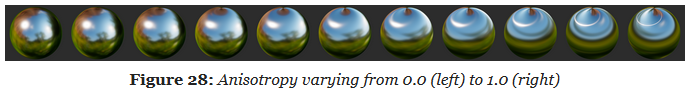
Anisotropy
Parameter
-
Amount of anisotropy.
-
Scalar
[-1..1]. -
Note that negative values will align the anisotropy with the bitangent direction instead of the tangent direction.
-
 .
.
-
For a rough metallic surface.
-
Anisotropy Specular BRDF
-
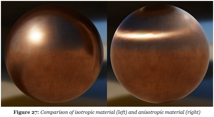
The standard material model described previously can only describe isotropic surfaces, that is, surfaces whose properties are identical in all directions. Many real-world materials, such as brushed metal, can, however, only be replicated using an anisotropic model.
-
 .
.
-
The Isotropic Specular BRDF described previously can be modified to handle anisotropic materials.
-
Burley's anisotropic NDF :
float at = max(roughness * (1.0 + anisotropy), 0.001); float ab = max(roughness * (1.0 - anisotropy), 0.001); float D_GGX_Anisotropic(float NoH, const vec3 h, const vec3 t, const vec3 b, float at, float ab) { float ToH = dot(t, h); float BoH = dot(b, h); float a2 = at * ab; highp vec3 v = vec3(ab * ToH, at * BoH, a2 * NoH); highp float v2 = dot(v, v); float w2 = a2 / v2; return a2 * w2 * w2 * (1.0 / PI); } -
Anisotropic visibility function
float at = max(roughness * (1.0 + anisotropy), 0.001);
float ab = max(roughness * (1.0 - anisotropy), 0.001);

float V_SmithGGXCorrelated_Anisotropic(float at, float ab, float ToV, float BoV,
        float ToL, float BoL, float NoV, float NoL) {
    float lambdaV = NoL * length(vec3(at * ToV, ab * BoV, NoV));
    float lambdaL = NoV * length(vec3(at * ToL, ab * BoL, NoL));
    float v = 0.5 / (lambdaV + lambdaL);
    return saturateMediump(v);
}
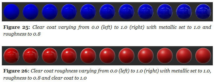
Clear Coat
Parameter
-
Clear Coat :
-
Strength of the clear coat layer.
-
Scalar
[0..1].
-
-
Clear Coat Roughness :
-
Perceived smoothness or roughness of the clear coat layer.
-
Scalar
[0..1].
-
-
 .
.
Clear Coat Specular BRDF
-
The standard material model is a good fit for isotropic surfaces made of a single layer.
-
Multi-layer materials are fairly common, particularly materials with a thin translucent layer over a standard layer.
-
Examples :
-
Car paints, soda cans, lacquered wood, acrylic, etc.
-
-
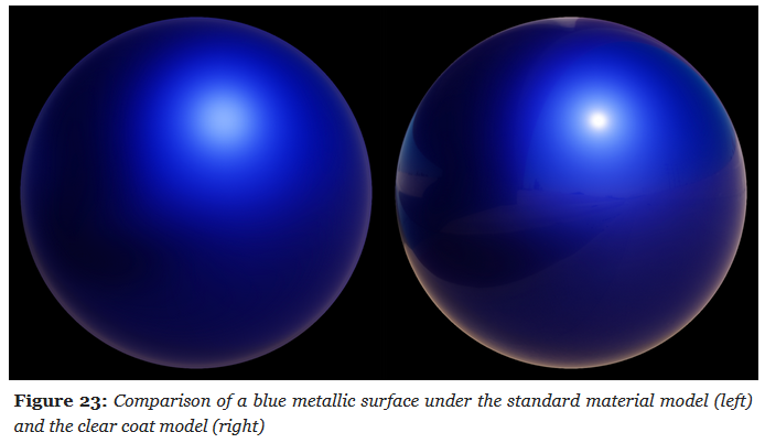 .
.
-
A clear coat layer can be simulated as an extension of the standard material model by adding a second specular lobe, which implies evaluating a second specular BRDF.
-
To simplify the implementation and parameterization, the clear coat layer will always be isotropic and dielectric.
-
Our model will however not simulate inter reflection and refraction behaviors.
-
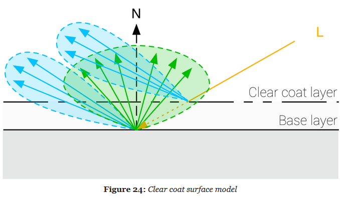 .
.
-
It's a Cook-Torrance specular microfacet model, with a GGX normal distribution function, a Kelemen visibility function, and a Schlick Fresnel function.
-
Kelemen visibility term :
float V_Kelemen(float LoH) {
    return 0.25 / (LoH * LoH);
}
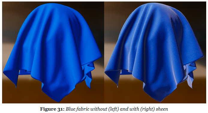
Sheen
Parameters
-
Color :
-
Specular tint to create two-tone specular fabrics (defaults to 0.04 to match the standard reflectance).
-
-
Subsurface Color :
-
Tint for the diffuse color after scattering and absorption through the material.
-
To create a velvet-like material, the base color can be set to black (or a dark color). Chromaticity information should instead be set on the sheen color. To create more common fabrics such as denim, cotton, etc. use the base color for chromaticity and use the default sheen color or set the sheen color to the luminance of the base color.
-
Cloth Specular BRDF
-
All the material models described previously are designed to simulate dense surfaces, both at a macro and at a micro level. Clothes and fabrics are however often made of loosely connected threads that absorb and scatter incident light. The microfacet BRDFs presented earlier do a poor job of recreating the nature of cloth due to their underlying assumption that a surface is made of random grooves that behave as perfect mirrors. When compared to hard surfaces, cloth is characterized by a softer specular lobe with a large falloff and the presence of fuzz lighting, caused by forward/backward scattering. Some fabrics also exhibit two-tone specular colors (velvets for instance).
-
A traditional microfacet BRDF fails to capture the appearance of a sample of denim fabric. The surface appears rigid (almost plastic-like), more similar to a tarp than a piece of clothing. This figure also shows how important the softer specular lobe caused by absorption and scattering is to the faithful recreation of the fabric.
-
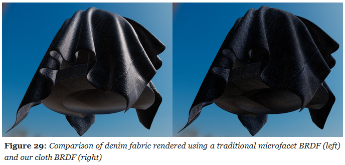 .
.
-
Velvet is an interesting use case for a cloth material model. As shown below, this type of fabric exhibits strong rim lighting due to forward and backward scattering. These scattering events are caused by fibers standing straight at the surface of the fabric. When the incident light comes from the direction opposite to the view direction, the fibers will forward-scatter the light. Similarly, when the incident light from the same direction as the view direction, the fibers will scatter the light backward.
-
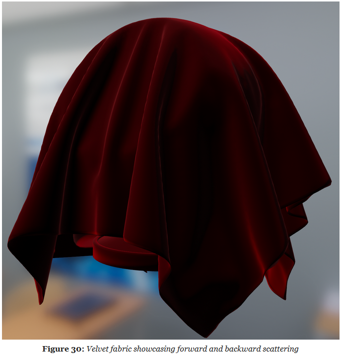 .
.
-
The cloth specular BRDF we use is a modified microfacet BRDF as described by Ashikhmin and Premoze .
-
Ashikhmin's Velvet NDF :
float D_Ashikhmin(float roughness, float NoH) { // Ashikhmin 2007, "Distribution-based BRDFs" float a2 = roughness * roughness; float cos2h = NoH * NoH; float sin2h = max(1.0 - cos2h, 0.0078125); // 2^(-14/2), so sin2h^2 > 0 in fp16 float sin4h = sin2h * sin2h; float cot2 = -cos2h / (a2 * sin2h); return 1.0 / (PI * (4.0 * a2 + 1.0) * sin4h) * (4.0 * exp(cot2) + sin4h); } -
Charlie NDF :
-
Optimized to properly fit in half float formats.
float D_Charlie(float roughness, float NoH) { // Estevez and Kulla 2017, "Production Friendly Microfacet Sheen BRDF" float invAlpha = 1.0 / roughness; float cos2h = NoH * NoH; float sin2h = max(1.0 - cos2h, 0.0078125); // 2^(-14/2), so sin2h^2 > 0 in fp16 return (2.0 + invAlpha) * pow(sin2h, invAlpha * 0.5) / (2.0 * PI); } -
Cloth Diffuse BRDF
-
Sheen :
-
To offer better control over the appearance of cloth and to give users the ability to recreate two-tone specular materials, we introduce the ability to directly modify the specular reflectance.
-
 .
.
-
-
Subsurface Scattering :
-
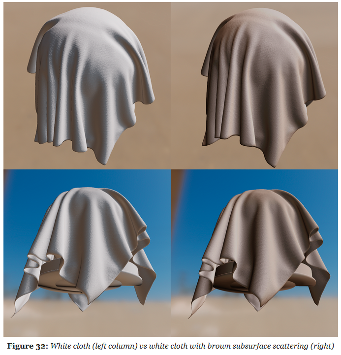 .
.
-
Direct Lighting
Parametrization
-
To simplify the implementation, all luminous powers will converted to luminous intensities () before being sent to the shader. The conversion is light dependent and is explained in the previous sections.
-
Type :
-
Directional, point, spot or area
-
Can be inferred from other parameters (e.g. a point light has a length, radius, inner angle and outer angle of 0).
-
-
Direction :
-
Used for directional lights, spot lights, photometric point lights, and linear and tubular area lights (orientation)
-
-
Color :
-
The color of emitted light, as a linear RGB color. Can be specified as an sRGB color or a color temperature in the tools
-
-
Intensity :
-
The light's brightness. The unit depends on the type of light
-
-
Falloff radius :
-
Maximum distance of influence
-
-
Inner angle :
-
Angle of the inner cone for spot lights, in degrees
-
-
Outer angle :
-
Angle of the outer cone for spot lights, in degrees
-
-
Length :
-
Length of the area light, used to create linear or tubular lights
-
-
Radius :
-
Radius of the area light, used to create spherical or tubular lights
-
-
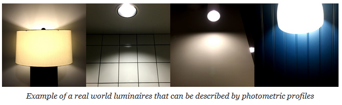
Photometric profile :
-
Texture representing a photometric light profile, works only for punctual lights
-
-
Masked profile :
-
Boolean indicating whether the IES profile is used as a mask or not. When used as a mask, the light's brightness will be multiplied by the ratio between the user specified intensity and the integrated IES profile intensity. When not used as a mask, the user specified intensity is ignored but the IES multiplier is used instead
-
-
Photometric multiplier :
-
Brightness multiplier for photometric lights (if IES as mask is turned off)
-
Color Temperature
-
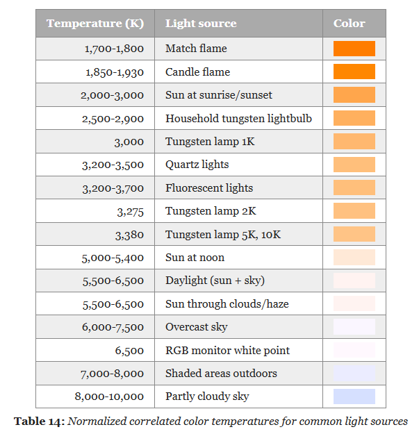 .
.
-
I got a little lost about this. See this session .
-
Convert from the XYZ space to linear RGB with a simple 3×3 matrix.
-
Conversion using the inverse matrix for the sRGB color space:
-
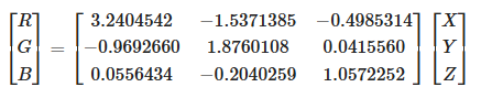 .
.
-
-
The result of these operations is a linear RGB triplet in the sRGB color space.
-
Since we care about the chromaticity of the results, we must apply a normalization step to avoid clamping values greater than 1.0 and distort resulting colors:
-
 .
.
-
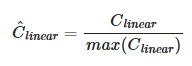
We must finally apply the sRGB opto-electronic conversion function (OECF) to obtain a displayable value (the value should remain linear if passed to the renderer for shading).
-
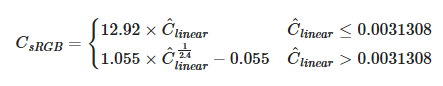 .
.
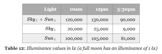
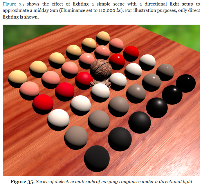
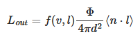
Directional Lights
-
The main purpose of directional lights is to recreate important light sources for outdoor environment, i.e. the sun and/or the moon. While directional lights do not truly exist in the physical world, any light source sufficiently far from the light receptor can be assumed to be directional
-
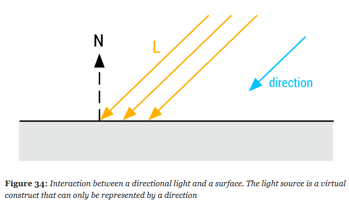 .
.
-
 .
.
-
Illuminance is measured with the unit Lux ($lx$); $lx$ is the symbol, like $W$ for Watts .
 .
.
-
-
Dynamic directional lights are particularly cheap to evaluate at runtime.
vec3 l = normalize(-lightDirection);
float NoL = clamp(dot(n, l), 0.0, 1.0);
// lightIntensity is the illuminance
// at perpendicular incidence in lux
float illuminance = lightIntensity * NoL;
vec3 luminance = BSDF(v, l) * illuminance;
Punctual Lights
-
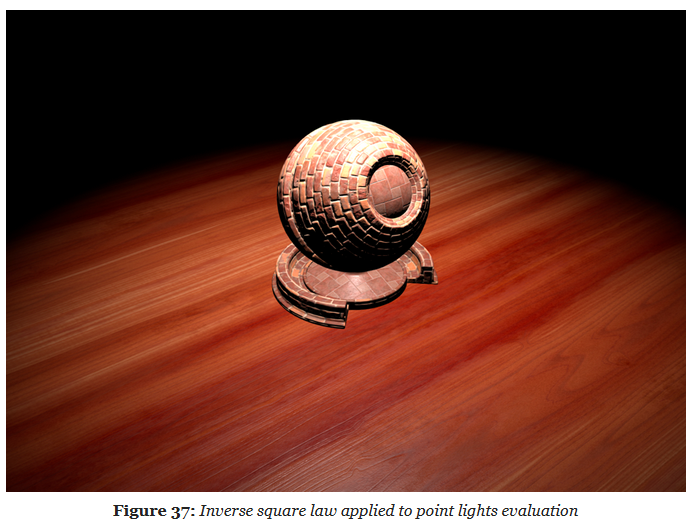
For punctual lights following the inverse square law, we use:
-
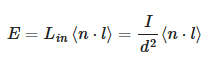 .
.
-
Where $d$ is the distance from a point at the surface to the light.
Point Lights
-
 .
.
-
 .
.
-
 .
.
-
Physically based punctual lights :
-
Note that the light intensity used in this piece of code is the luminous intensity in , converted from the luminous power CPU-side. This snippet is not optimized and some of the computations can be offloaded to the CPU (for instance the square of the light's inverse falloff radius, or the spot scale and angle).
float getSquareFalloffAttenuation(vec3 posToLight, float lightInvRadius) { float distanceSquare = dot(posToLight, posToLight); float factor = distanceSquare * lightInvRadius * lightInvRadius; float smoothFactor = max(1.0 - factor * factor, 0.0); return (smoothFactor * smoothFactor) / max(distanceSquare, 1e-4); } float getSpotAngleAttenuation(vec3 l, vec3 lightDir, float innerAngle, float outerAngle) { // the scale and offset computations can be done CPU-side float cosOuter = cos(outerAngle); float spotScale = 1.0 / max(cos(innerAngle) - cosOuter, 1e-4) float spotOffset = -cosOuter * spotScale float cd = dot(normalize(-lightDir), l); float attenuation = clamp(cd * spotScale + spotOffset, 0.0, 1.0); return attenuation * attenuation; } vec3 evaluatePunctualLight() { vec3 l = normalize(posToLight); float NoL = clamp(dot(n, l), 0.0, 1.0); vec3 posToLight = lightPosition - worldPosition; float attenuation; attenuation = getSquareFalloffAttenuation(posToLight, lightInvRadius); attenuation *= getSpotAngleAttenuation(l, lightDir, innerAngle, outerAngle); vec3 luminance = (BSDF(v, l) * lightIntensity * attenuation * NoL) * lightColor; return luminance; } vec3 l = normalize(-lightDirection); float NoL = clamp(dot(n, l), 0.0, 1.0); // lightIntensity is the illuminance // at perpendicular incidence in lux float illuminance = lightIntensity * NoL; vec3 luminance = BSDF(v, l) * illuminance; -
Spot Lights
-
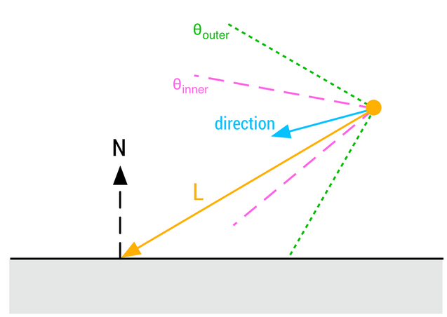 .
.
-
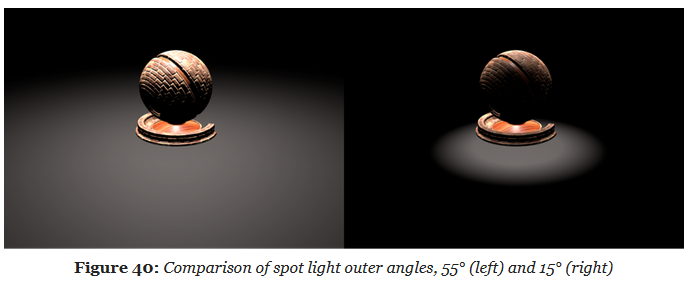
-
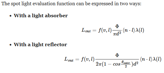 .
.
Photometric Lights
-
 .
.
-
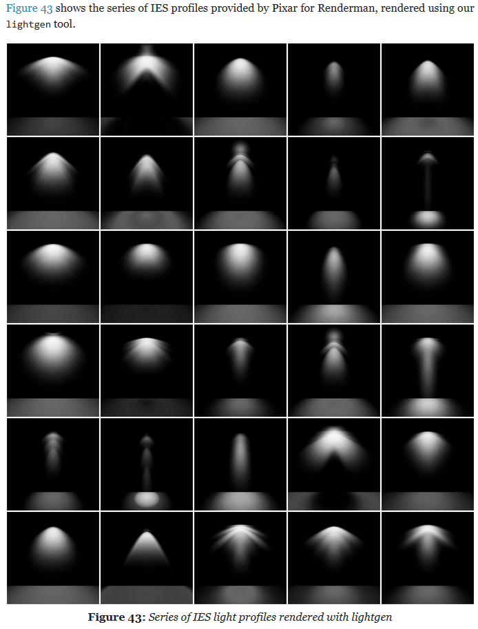 .
.
-
Implementation:
float getPhotometricAttenuation(vec3 posToLight, vec3 lightDir) {
    float cosTheta = dot(-posToLight, lightDir);
    float angle = acos(cosTheta) * (1.0 / PI);
    return texture2DLodEXT(lightProfileMap, vec2(angle, 0.0), 0.0).r;
}

vec3 evaluatePunctualLight() {
    vec3 l = normalize(posToLight);
    float NoL = clamp(dot(n, l), 0.0, 1.0);
    vec3 posToLight = lightPosition - worldPosition;

    float attenuation;
    attenuation  = getSquareFalloffAttenuation(posToLight, lightInvRadius);
    attenuation *= getSpotAngleAttenuation(l, lightDirection, innerAngle, outerAngle);
    attenuation *= getPhotometricAttenuation(l, lightDirection);
        // This is the addition to the Punctual Light. It requires a lightProfileMap, etc.

    float luminance = (BSDF(v, l) * lightIntensity * attenuation * NoL) * lightColor;
    return luminance;
}
-
The light intensity is computed CPU-side and depends on whether the photometric profile is used as a mask.
float multiplier;
// Photometric profile used as a mask
if (photometricLight.isMasked()) {
    // The desired intensity is set by the artist
    // The integrated intensity comes from a Monte-Carlo
    // integration over the unit sphere around the luminaire
    multiplier = photometricLight.getDesiredIntensity() /
            photometricLight.getIntegratedIntensity();
} else {
    // Multiplier provided for convenience, set to 1.0 by default
    multiplier = photometricLight.getMultiplier();
}

// The max intensity in cd comes from the IES profile
float lightIntensity = photometricLight.getMaxIntensity() * multiplier;
Mobile Adaptations
Pre-Expose Lights
-
"How to store and handle the large range of values produced by the lighting code?"
-
Assuming computations performed at full precision in the shaders, we still want to be able to store the linear output of the lighting pass in a reasonably sized buffer (
RGB16For equivalent). -
The most obvious and easiest way to achieve this is to simply apply the camera exposure before writing out the result of the lighting pass.
-
Pre-exposing lights allows the entire shading pipeline to use half precision floats.
-
In practice we pre-expose the following lights:
-
Punctual lights (point and spot):
-
on the GPU
-
-
Directional light:
-
on the CPU
-
-
IBLs:
-
on the CPU
-
-
Material emissive:
-
on the GPU
-
-
-
This can be easily done with:
fragColor = luminance * camera.exposure;
-
But, this requires intermediate computations to be performed with single precision floats.
-
We would instead prefer to perform all (or at least most) of the lighting work using half precision floats instead.
-
Doing so can greatly improve performance and power usage, particularly on mobile devices. Half precision floats are however ill-suited for this kind of work as common illuminance and luminance values (for the sun for instance) can exceed their range.
-
The solution is to simply pre-expose the lights themselves instead of the result of the lighting pass.
-
This can be done efficiently on the CPU if updating a light's constant buffer is cheap.
-
This can also be done on the GPU , like so:
// The inputs must be highp/single precision,
// both for range (intensity) and precision (exposure)
// The output is mediump/half precision
float computePreExposedIntensity(highp float intensity, highp float exposure) {
    return intensity * exposure;
}

Light getPointLight(uint index) {
    Light light;
    uint lightIndex = // fetch light index;

    // the intensity must be highp/single precision
    highp vec4 colorIntensity  = lightsUniforms.lights[lightIndex][1];

    // pre-expose the light
    light.colorIntensity.w = computePreExposedIntensity(
            colorIntensity.w, frameUniforms.exposure);

    return light;
}
Shadows
Shadow Map
-
"The scene is first rendered at the point of view of the light, and the result of that image is stored in a image called Shadow Map".
-
It stores the depth map.
-
-
"If the light source doesn't 'see' something, then color the pixel dark".
-
The final result is a pixelated shadow. To improve this, PCF (Percentage Closer Filtering) can be done.
-
4x4 PCF is ok, but adding offsets helps in randomness and makes the effect more natural.
-
-
"You want the shadow area to be smallest as possible, while containing all the objects in the camera's view frustum".
-
-
The following techniques are implemented:
-
Cascaded Shadow Maps
-
Stabilized Cascaded Shadow Maps
-
Automatic Cascade Fitting based on depth buffer analysis, as in Sample Distribution Shadow Maps .
-
Various forms of Percentage Closer Filtering
-
Exponential Variance Shadow Maps (EVSM).
-
-
-
Improved shadows using dithering and temporal supersampling .
Percentage Closer Filtering (PCF)
-
.
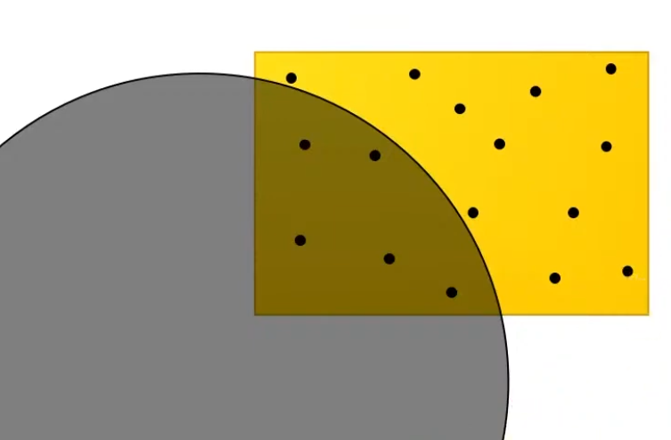
Soft-Shadows
-
Usual for area lights.
-
 .
.
-
 .
.
-
We will not do proper shading from this light source, but only compute what percentage of the area of the light is covered.
Raytracing
-
It's the proper way to solve it, but it's costly; the other techniques are approximations.
-
Send rays from the point to the light source.
-
 .
.
-
Approximate the percentage of the area that is visible to the light source, via the ratio of rays that hit the light vs rays that didn't hit the light.
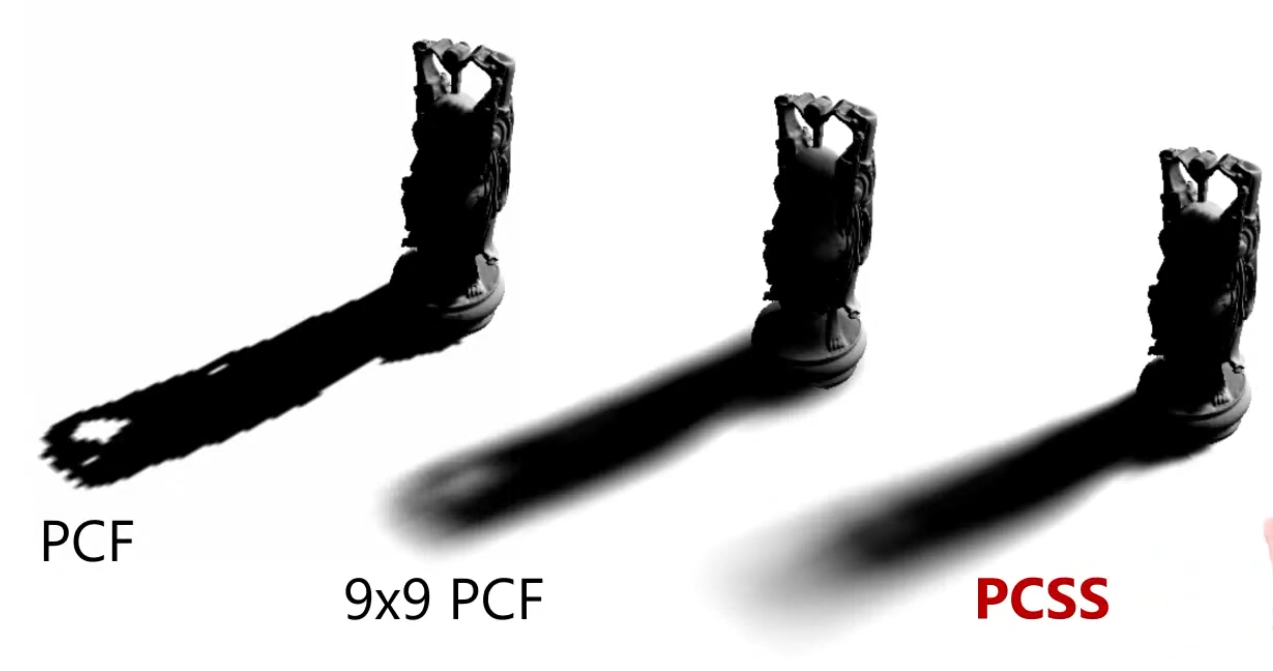
Percentage Closer Soft Shadows (PCSS)
-
Presented at Siggraph in 2005.
-
 .
.
-
The PCF sample varies through out the shadow, so the shadows closer to the object look sharp and far away from the object look smooth.
-
Based on the distance to the object from the floor, you decide what filter you should use.
-
How far the occluder is vs how far the point I want to compute is.
-
It also uses the occluder size.
-
 .
.
-
-
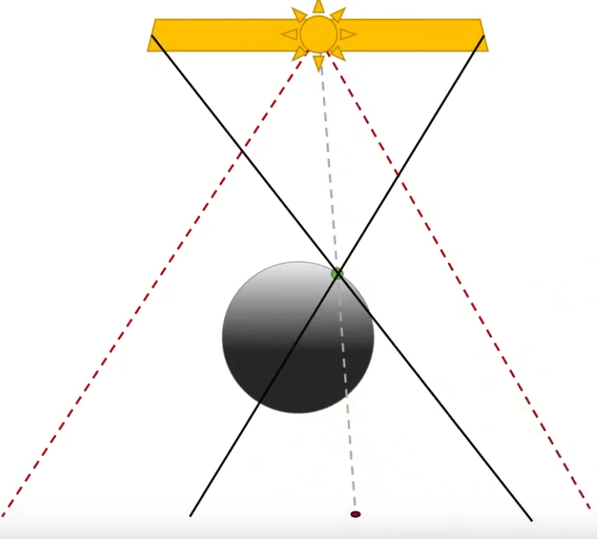
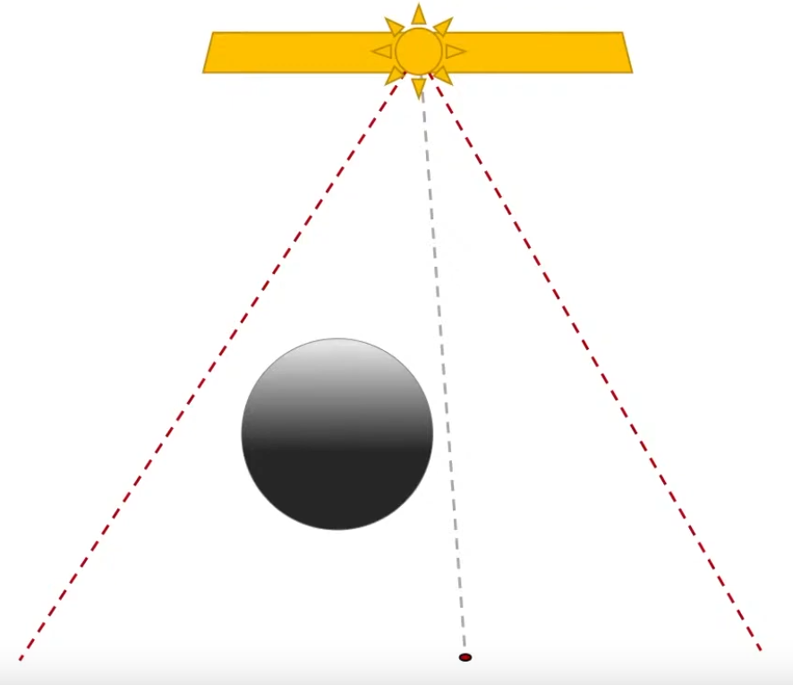
Requires a 'Occluder Search' so a situation like below correctly indicates that should be shadow in that point.
-
The shadow in that points comes from the fact that the left side of the light source blocks the object.
-
 .
.
-
-
As PCSS requires Occluder Search and a PCF with large radius, depending on the situation, this method of soft shadows is not cheap.
-
Is cheaper than tracing rays, tho.
-
-
 .
.
~Other Techiniques
-
Doesn't work with Shadow Maps, as Shadow Maps just gives you a blunt occlusion information.
-
Tries to approximate the PCF / PCSS, for soft-shadows instead of computing it.
-
Variance Shadow Maps (VSM) .
-
-
Convolution Shadow Maps (CSM) .
-
-
Exponential Shadow Maps (ESM) .
-
-
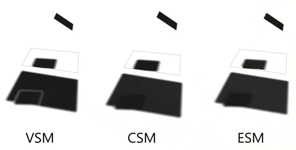 .
.
-
There are improvements to these methods, trying to solve the problems of these approximations.
Radiance Cascades
-
I saw a video demonstrating the usage of radiance cascades for soft-shadows.
Skybox / Skydome
-
Steps to reproduce the Skybox from the Vulkan sample HDR:
-
Load KTX file.
-
See
api_vulkan_sample.cpp->load_texture_cubemap (1202).
-
-
In:
in_pos(vec3). -
Desc Sets: Camera View and Camera Proj in the shader
-
out:
out_uvw(vec3) andout_pos(vec3).
textures.envmap = load_texture_cubemap("textures/uffizi_rgba16f_cube.ktx", vkb::sg::Image::Color);

vkb::initializers::write_descriptor_set(descriptor_sets.object, VK_DESCRIPTOR_TYPE_UNIFORM_BUFFER, 0, &matrix_buffer_descriptor),
vkb::initializers::write_descriptor_set(descriptor_sets.object, VK_DESCRIPTOR_TYPE_COMBINED_IMAGE_SAMPLER, 1, &environment_image_descriptor),
// Vertex layout (location = 0) in vec3 inPos; layout (binding = 0) uniform UBO { mat4 projection; // camera.matrices.perspective; mat4 skybox_modelview; // camera.view } ubo; layout (location = 0) out vec3 outUVW; layout (location = 1) out vec3 outPos; outUVW = inPos; outPos = vec3(mat3(ubo.skybox_modelview) * inPos); gl_Position = vec4(ubo.projection * vec4(outPos, 1.0)); // Frag layout (binding = 1) uniform samplerCube samplerEnvMap; layout (location = 0) in vec3 inUVW; layout (location = 0) out vec4 outColor0; vec3 normal = normalize(inUVW); color = texture(samplerEnvMap, normal); // Color with manual exposure into attachment 0 outColor0.rgb = vec3(1.0) - exp(-color.rgb * ubo.exposure); -
-
See UI and Skybox from Kohi Engine.-
Yea.. The engine is an insane mess.
-
The shaders are confusing and use the camera matrix and model matrix to draw UI, wtf.
-
It's impossible to find out how the graphics pipeline is created. It's an infinite wormhole.
-
Transparency
Alpha
// baseColor has already been premultiplied
vec4 shadeSurface(vec4 baseColor) {
    float alpha = baseColor.a;

    vec3 diffuseColor = evaluateDiffuseLighting();
    vec3 specularColor = evaluateSpecularLighting();

    return vec4(diffuseColor + specularColor, alpha);
}
Alpha Blend
-
With Z-Buffer Rasterization, the order matters.
-
 .
.
-
If renderer back to front, it works fine.
-
-
 .
.
-
With A-Buffer Rasterization, the objects get sorted based on the alpha, so we don't have this problem.
-
GPUs use Z-Buffer, so we are stuck with it.
-
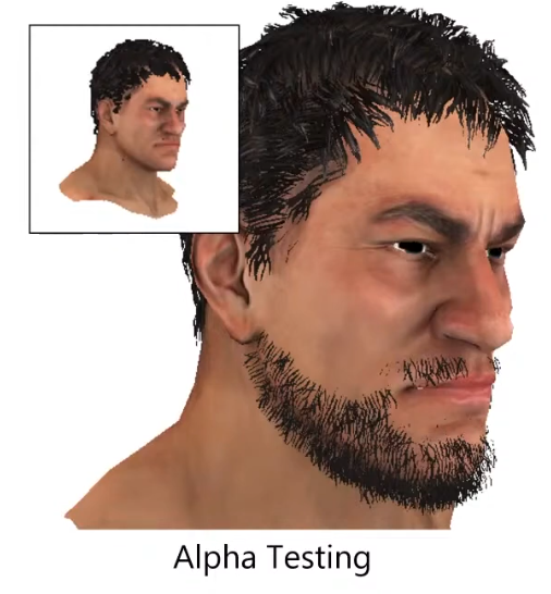
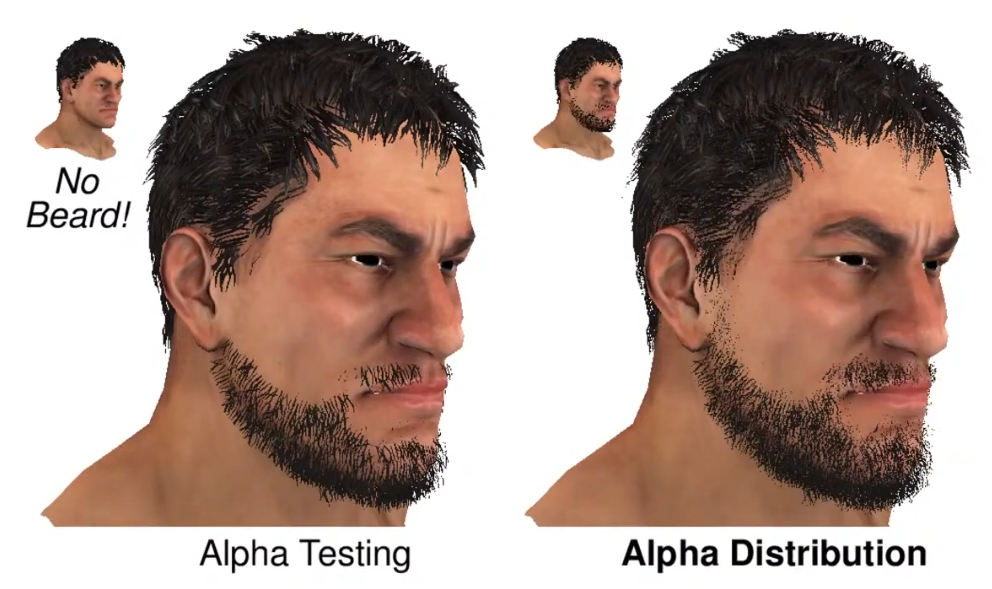
Alpha Testing
-
 .
.
-
If the alpha is below a certain threshold, discard.
-
Alpha Testing with mipmapping can have problems:
-
 .
.
-
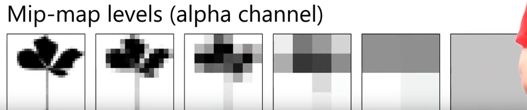 .
.
-
The alpha ends up converging to a value below the threshold
-
 .
.
-
At far away, the character loses its beard.
-
-
Hashed Alpha Testing
-
-
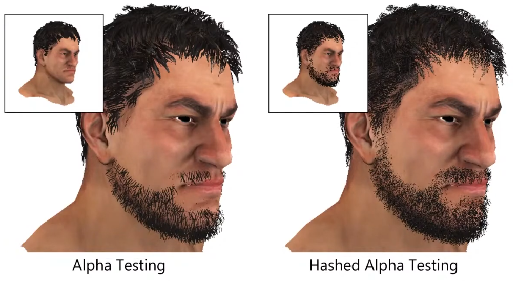 .
.
-
Test randomly.
-
The discard is made in software, not in hardware.
-
It's really noise, as it looks like dithering.
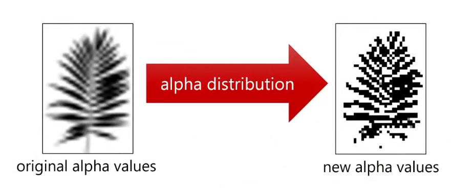
Alpha Distribution
-
-
 .
.
-
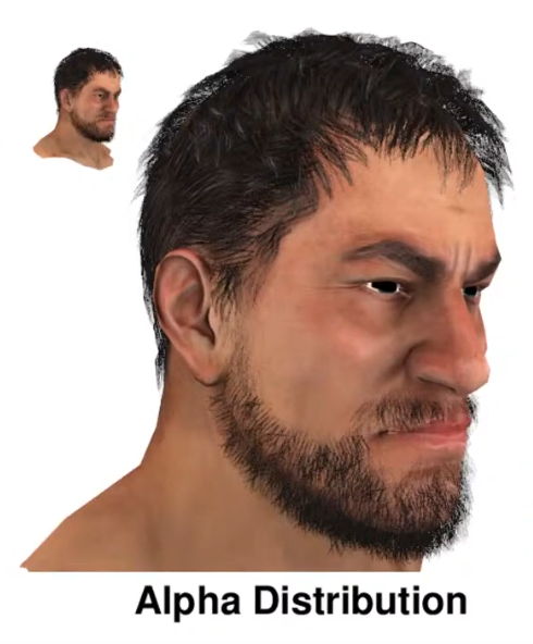 - Alpha Distribution + Alpha to Coverage.
-
Uses dithering first.
-
 .
.
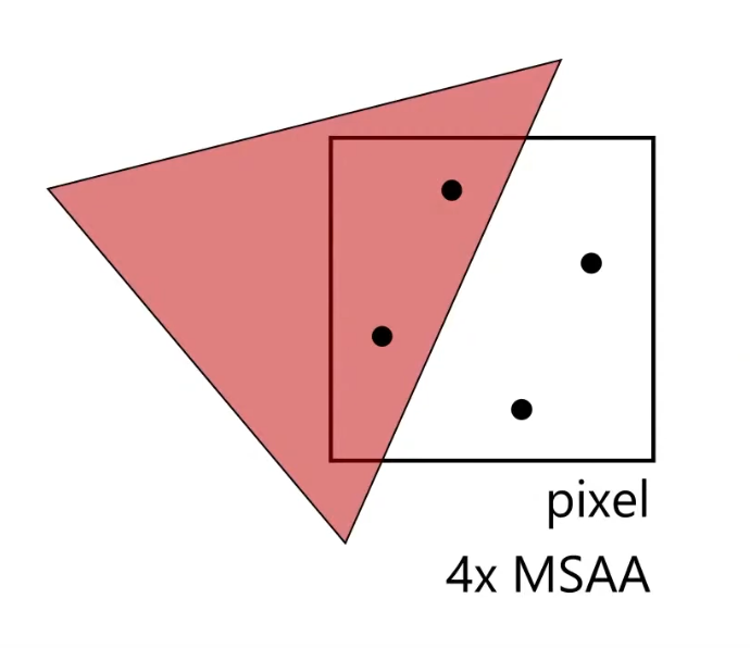
Alpha to Coverage
-
 .
.
-
You get smoother pixels than with Alpha Testing.
-
It adds different values of alpha, instead of 0 or 1.
-
With 4x, you can get 4 different values of alpha: 0.0, 0.25, 0.5, 0.75.
-
-
 .
.
-
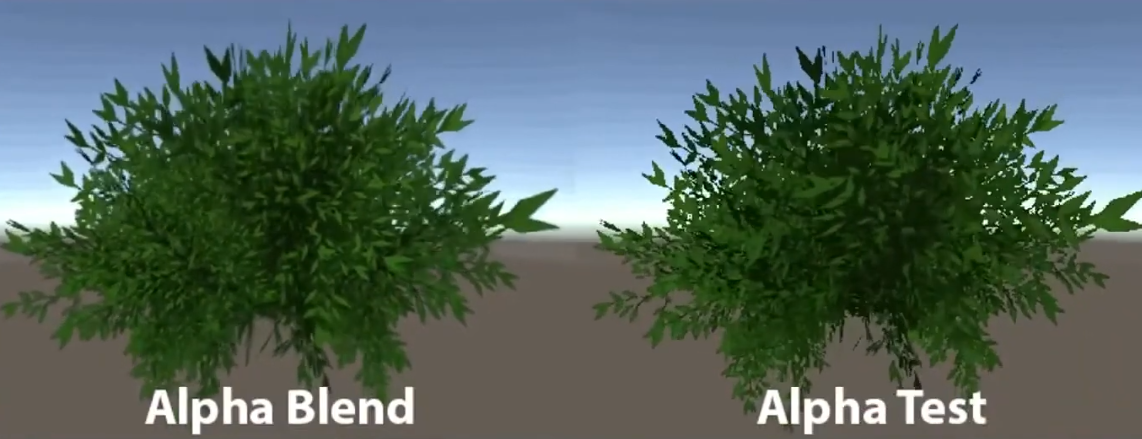
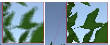
Alpha to Coverage (left), Alpha Testing (right).
-
Order-Independent Transparency
-
Godot 4 - Render Limitations .
-
Godot doesn't do OIT.
-
The article shows how to deal with it.
-
Depth Peeling
-
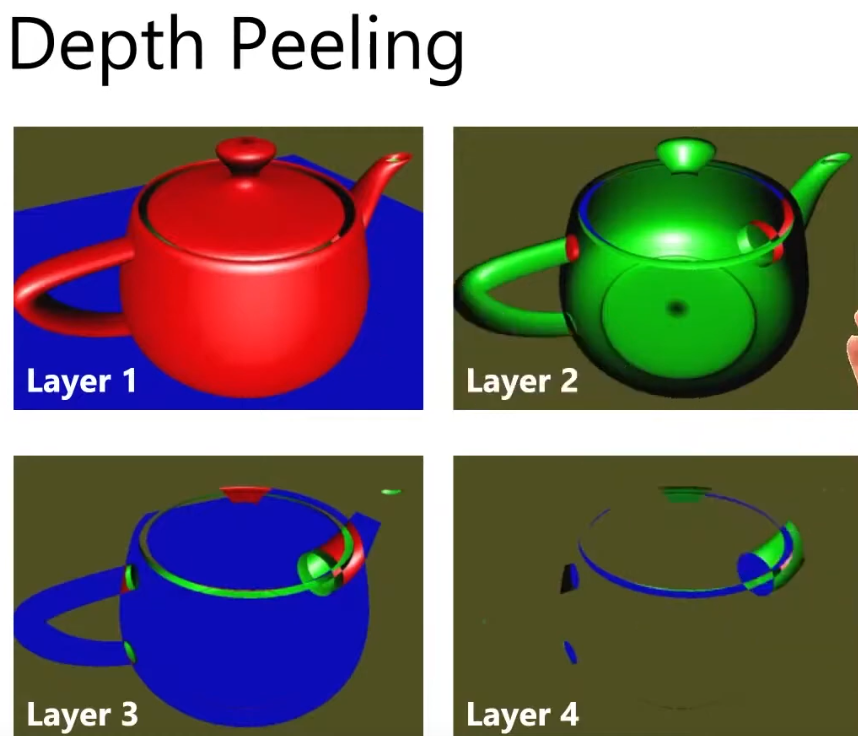
-
Layer 1:
-
Render as full opaque.
-
-
Layer 2:
-
Use the depth buffer from Layer 1 to perform additional depth test while rendering Layer 2.
-
-
Etc, etc.
-
The amount of layers depend on the object.
-
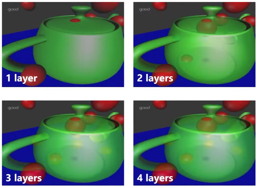 .
.
-
For every layer, you have to render the scene again; 4 layers = 4 times the cost.
"Software A-Buffer"
-
To avoid the costs of Depth Peeling, we soft-implement A-Buffer.
-
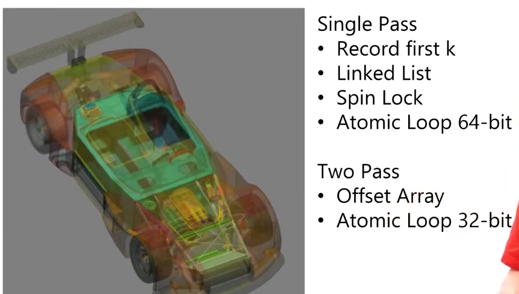 .
.
-
"Order-Independent Transparency in OpenGL 4.X - Nvidia".
Refraction
-
You need to know the light that is coming from behind the surface.
-
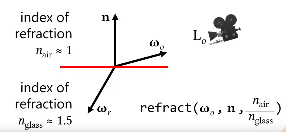 .
.
-
The front and back need to be considered.
-
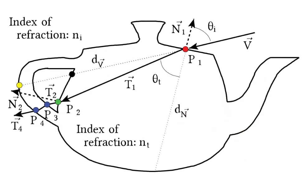 .
.
-
The rays refract in and out.
-
-
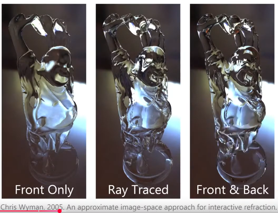 .
.
-
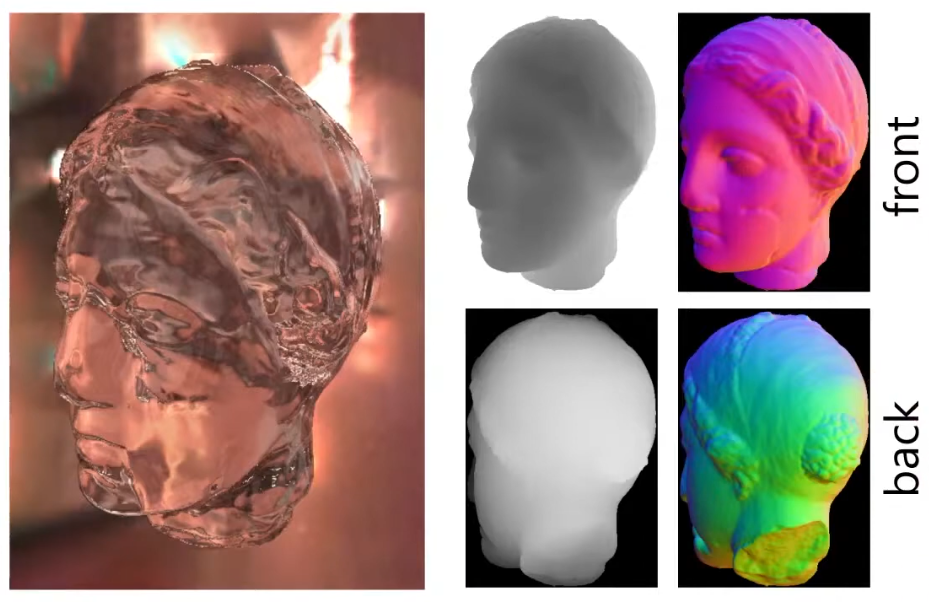 .
.
-
A normal render gives you the depth and normals of the front.
-
We render the back as a pre-pass, to get the depth and normals of the back.
-
The difference between the depth value from the back and the front will give you the thickness of the object.
-
This is an approximation for how long the ray will travel inside that object.
-
"If I were to travel this much, where will I end up in the Back texture?".
-
This gives you the direction of the exiting ray, so you can sample an environment map.
-
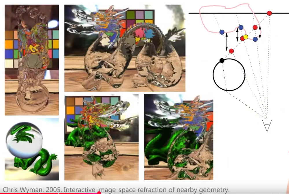 .
.
-
To see other objects, besides the environment map, the objects need to be rendered first, etc; a process similar to parallax mapping is used to solve this.
-
Super fast, cool.
Global Illumination / Indirect Lighting
-
A broad term that refers to any algorithm or technique that simulates how light bounces around a scene, not just directly from light sources but also after interactions with surfaces.
-
It encompasses both direct lighting (light coming straight from a source) and indirect lighting (light that has bounced one or more times).
Terms
Irradiance
-
Irradiance (scalar) :
-
At a surface point, the integral of incoming radiance over the hemisphere (units: W/m²).
-
Often the quantity of interest for diffuse shading.
-
-
Irradiance field :
-
An Irradiance Field is the continuous phenomenon.
-
A function that maps spatial position (and sometimes orientation) to irradiance.
-
In papers this term can mean the true continuous field, or a specific continuous representation (e.g., a voxel grid, analytic basis, or neural field).
-
-
Irradiance probes :
-
An Irradiance Probe is a discrete measurement of that phenomenon.
-
A set of sampled measurements placed at discrete spatial locations.
-
Each probe stores an irradiance representation (examples: spherical-harmonic coefficients, a small cubemap, or directional coefficients).
-
During rendering the scene samples/interpolates between probes to approximate the irradiance at arbitrary points.
-
Techniques
-
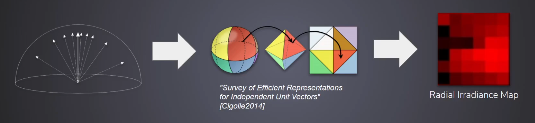
-
Appeared in Surfels.
-
Parameterizations / sampling layouts for the sphere
Octahedral Maps
-
A bijective mapping (with a fold) that encodes a unit 3D direction
n = (x,y,z)into 2D texture coordinatesu,v ∈ [0,1]. -
Designed to pack the sphere into a single square texture with less angular distortion than latitude–longitude and usually fewer wasted texels than cube maps.
-
Commonly used to store normals, unit vectors (reflection vectors, tangent-space directions), or per-direction scalar/vector fields (e.g., an environment map sampled per texel).
Cube Maps
-
Precomputing $L_{DFG}$ :
-
The term $L_{DFG}$ is only dependent on $n.v$. Below, the normal is arbitrarily set to $n = [0, 0, 1]$ and $v$ is chosen to satisfy $n.v$. The vector $h_i$ is the $D_{GGX}(\alpha)$ important direction sample $i$.
float GDFG(float NoV, float NoL, float a) { float a2 = a * a; float GGXL = NoV * sqrt((-NoL * a2 + NoL) * NoL + a2); float GGXV = NoL * sqrt((-NoV * a2 + NoV) * NoV + a2); return (2 * NoL) / (GGXV + GGXL); } float2 DFG(float NoV, float a) { float3 V; V.x = sqrt(1.0f - NoV*NoV); V.y = 0.0f; V.z = NoV; float2 r = 0.0f; for (uint i = 0; i < sampleCount; i++) { float2 Xi = hammersley(i, sampleCount); float3 H = importanceSampleGGX(Xi, a, N); float3 L = 2.0f * dot(V, H) * H - V; float VoH = saturate(dot(V, H)); float NoL = saturate(L.z); float NoH = saturate(H.z); if (NoL > 0.0f) { float G = GDFG(NoV, NoL, a); float Gv = G * VoH / NoH; float Fc = pow(1 - VoH, 5.0f); r.x += Gv * (1 - Fc); r.y += Gv * Fc; } } return r * (1.0f / sampleCount); } -
-
Filament Engine coordinates system :
-
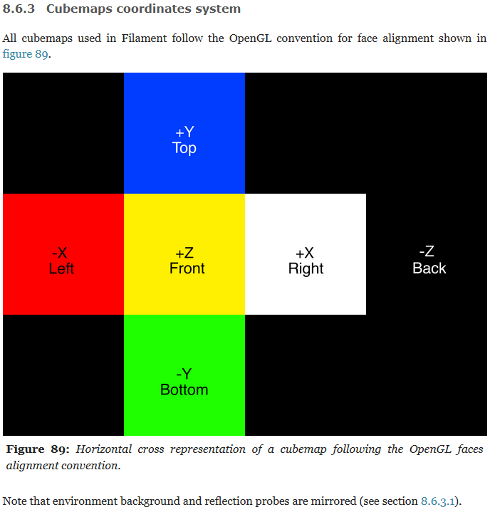 .
.
-
To simplify the rendering of reflections, IBL cubemaps are stored mirrored on the X axis. This is the default behaviour of the
cmgentool. This means that an IBL cubemap used as environment background needs to be mirrored again at runtime. An easy way to achieve this for skyboxes is to use textured back faces. Filament does this by default. -
To convert equirectangular environment maps to horizontal/vertical cross cubemaps we position the +Z face in the center of the source rectilinear environment map.
-
When specifying a skybox or an IBL in Filament, the specified cubemap is oriented such that its -Z face points towards the +Z axis of the world (this is because filament assumes mirrored cubemaps). However, because environments and skyboxes are expected to be pre-mirrored, their -Z (back) face points towards the world's -Z axis as expected (and the camera looks toward that direction by default).
-
Directional Data (Represent or approximate functions on the sphere (bases or parametric lobes))
-
SG Series Part 1: A Brief (and Incomplete) History of Baked Lighting Representations .
-
Sounds very interesting and relevant.
-
When an SH/SG/wavelet can “replace” a cubemap/oct map — and when it cannot
-
Replace (acceptable / typical):
-
Low-frequency lighting (diffuse irradiance): SH (low-order) is commonly used instead of sampling a full cubemap at runtime because SH compactly encodes low-frequency content and allows analytic convolution with Lambertian cosine. That avoids per-pixel cubemap lookups for diffuse IBL.
-
Compact specular approximation: Representing an environment by a small number of SG lobes can replace a cubemap for fast approximate glossy shading or importance sampling when the environment is lobe-like.
-
Compression / streaming: Wavelets (or hierarchical transforms) can replace a naive cubemap storage by providing a compressed, multiresolution representation that is progressively refinable.
-
-
Cannot fully replace (or will be lossy / expensive to use):
-
Detailed, high-frequency reflections (sharp mirror-like): Full-resolution cubemap/oct textures or prefiltered mipmap chains (PMREM) are the usual approach. SH needs very high band count (many coefficients) to represent sharp features, and SG requires many lobes to approximate complex high-frequency structure — both become expensive or inaccurate.
-
Arbitrary sampling and filtering: A texture parameterization (cubemap/oct) is a direct sampling representation and is straightforward to sample, filter (with caveats) and prefilter with hardware. Basis expansions require projection and reconstruction steps before sampling in the standard pipeline.
-
Haar Wavelets
-
A family of localized, multiresolution basis functions (Haar is the simplest wavelet) that represent signals with coarse-to-fine detail. Haar wavelets are piecewise-constant, have compact support, and provide spatial locality and hierarchical decomposition.
-
Typical form (1D/2D idea): scaling functions and wavelet functions that split signal into averages + differences at successive scales. On the sphere one can build analogous spherical wavelet bases (e.g., via hierarchical partitioning of the sphere).
-
Properties: spatially localized, multi-resolution (supports progressive refinement), good at representing localized/high-frequency features and discontinuities, many coefficients are zero or small for sparse signals, not globally smooth (Haar is discontinuous). Wavelet transforms can be fast (O(n)). Rotation is awkward for bases tied to a fixed partitioning.
-
Common graphics uses: compression and multi-resolution representation of environment maps or textures, adaptive shading, fast hierarchical importance sampling / level-of-detail, GPU-friendly encodings, and sparse approximations of signals with local sharp features.
-
Trade-offs: better for localized/high-frequency structure and compression; Haar specifically is low-order (blocky) unless higher-order wavelets are used; rotation and analytic convolution are not generally simple in the wavelet domain without additional structure.
Spherical Gaussians (SG)
-
What it is (short): parametric, localized “lobe” functions on the sphere that approximate a single-peaked angular distribution (an axis-aligned Gaussian-like lobe).
-
Typical form (common form): $G(\omega;\mu,\kappa)=\exp\big(\kappa(\mu\cdot\omega-1)\big)$, where $\mu$ is the lobe axis and $\kappa$ (or similar) controls concentration (larger $\kappa$ = narrower lobe). (Different papers use slightly different normalization/scales.)
-
Properties: strongly localized, easily rotated by changing $\mu$, analytic approximations exist for products and convolutions with some BRDF lobes (useful approximations), compact parametric representation (axis + sharpness), cheap evaluation of a single lobe. Not an orthogonal basis. Multiple SGs can be summed to approximate complex lobes.
-
Common graphics uses: representing specular lobes and glossy reflections, analytic or semi-analytic shading and convolution approximations, importance sampling, fitting environment lighting with a sum of lobes for real-time shading. SGs are also used in prefiltered environment maps where single-lobe behavior is important.
-
Trade-offs: simple and efficient for localized lobes; approximating arbitrary functions requires many SGs; not linear-orthonormal (so projection/coefficients don’t have the same algebraic niceties as SH).
Spherical Harmonics (SH)
-
An Efficient Representation for Irradiance Environment Maps - Ramamoorthi & Hanrahan - Siggraph 2001 .
-
Frequency Space Environment Map Rendering - Ramamoorthi & Hanrahan- Siggraph 2002 .
-
"Spherical harmonic reflection map (SHRM)".
-
-
Lighting and Material of Halo 3 - Siggraph 2008 .
-
Bungie pioneered baked SH lighting in a shipped game with Halo 3 (Xbox 360, 2007). Halo 3’s engine precomputed “light probe” textures: each texel stored multiple SH coefficients (the slides cite 9–16 floats per texel) representing the incoming diffuse light at that point. These SH lightmaps were then sampled in shaders, so that static geometry received baked global illumination, and dynamic models could be lit by dot-producting their SH transfer vectors against the light-probe SH. (Siggraph 2008 “Lighting and Materials of Halo 3” notes SH lightmaps as a natural extension of lightmaps.
-
-
Filament - Spherical Harmonics .
-
C++ implementation to compute a non-normalized SH basis:
static inline size_t SHindex(ssize_t m, size_t l) { return l * (l + 1) + m; } void computeShBasis( double* const SHb, size_t numBands, const vec3& s) { // handle m=0 separately, since it produces only one coefficient double Pml_2 = 0; double Pml_1 = 1; SHb[0] = Pml_1; for (ssize_t l = 1; l < numBands; l++) { double Pml = ((2 * l - 1) * Pml_1 * s.z - (l - 1) * Pml_2) / l; Pml_2 = Pml_1; Pml_1 = Pml; SHb[SHindex(0, l)] = Pml; } double Pmm = 1; for (ssize_t m = 1; m < numBands ; m++) { Pmm = (1 - 2 * m) * Pmm; double Pml_2 = Pmm; double Pml_1 = (2 * m + 1)*Pmm*s.z; // l == m SHb[SHindex(-m, m)] = Pml_2; SHb[SHindex( m, m)] = Pml_2; if (m + 1 < numBands) { // l == m+1 SHb[SHindex(-m, m + 1)] = Pml_1; SHb[SHindex( m, m + 1)] = Pml_1; for (ssize_t l = m + 2; l < numBands; l++) { double Pml = ((2 * l - 1) * Pml_1 * s.z - (l + m - 1) * Pml_2) / (l - m); Pml_2 = Pml_1; Pml_1 = Pml; SHb[SHindex(-m, l)] = Pml; SHb[SHindex( m, l)] = Pml; } } } double Cm = s.x; double Sm = s.y; for (ssize_t m = 1; m <= numBands ; m++) { for (ssize_t l = m; l < numBands; l++) { SHb[SHindex(-m, l)] *= Sm; SHb[SHindex( m, l)] *= Cm; } double Cm1 = Cm * s.x - Sm * s.y; double Sm1 = Sm * s.x + Cm * s.y; Cm = Cm1; Sm = Sm1; } }-
C++ code to compute $\hat{C}_l$:
static double factorial(size_t n, size_t d = 1); // < cos(theta) > SH coefficients pre-multiplied by 1 / K(0,l) double computeTruncatedCosSh(size_t l) { if (l == 0) { return M_PI; } else if (l == 1) { return 2 * M_PI / 3; } else if (l & 1) { return 0; } const size_t l_2 = l / 2; double A0 = ((l_2 & 1) ? 1.0 : -1.0) / ((l + 2) * (l - 1)); double A1 = factorial(l, l_2) / (factorial(l_2) * (1 << l)); return 2 * M_PI * A0 * A1; } // returns n! / d! double factorial(size_t n, size_t d ) { d = std::max(size_t(1), d); n = std::max(size_t(1), n); double r = 1.0; if (n == d) { // intentionally left blank } else if (n > d) { for ( ; n>d ; n--) { r *= n; } } else { for ( ; d>n ; d--) { r *= d; } r = 1.0 / r; } return r; } -
-
Basis functions $Y_{\ell}^m(\theta,\phi)$ indexed by degree $\ell\ge 0$ and order $-\ell\le m\le\ell$. A function $f(\omega)$ on the sphere is expanded as $f(\omega)=\sum_{\ell=0}^{L}\sum_{m=-\ell}^{\ell} c_{\ell m} Y_{\ell}^m(\omega)$.
-
Are an orthonormal basis for functions on the sphere. In real-time lighting they are used to compactly represent low-frequency angular functions (environment illumination, visibility, convolution kernels).
-
Irradiance probes commonly store SH coefficients so the renderer can approximate diffuse lighting quickly.
-
Why is it useful for Irradiance / Probes :
-
Compression : low-frequency lighting (diffuse environment lighting, soft shadows) is well-approximated by a small number of SH bands (e.g. 9 coefficients).
-
Linear projection : you can project an environment (cubemap, sampling) onto SH. Once you have certain coefficients, you store those in a probe instead of storing a full cubemap.
-
Fast evaluation : to evaluate the approximated radiance or irradiance at some direction $\omega$, evaluate the SH basis at $\omega$ and form the dot product with coefficients: $f(\omega)=\sum a_{l}^{m}Y_{l}^{m}(\omega)$. That dot product is inexpensive for small L.
-
Convolution property (why diffuse works well) : for Lambertian reflection you need the cosine-weighted integral of incoming radiance. The cosine kernel is low-frequency and its SH representation has non-zero weight only on low bands. Convolving $L_i$ with the cosine kernel reduces to scaling SH bands by precomputed factors. Practically, this means you can compute irradiance from the projected SH coefficients cheaply without re-sampling the entire environment at render time.
-
-
-
A demonstration of spherical harmonics used to construct the surface of the earth at increasing angular resolution.
-
-
Spherical Harmonics Visualization .
-
We describe the possible fundamental vibrations on a sphere in three dimensions by counting, mirroring and rotating nodal lines.
-
-
-
Idk, wtf.
-
-
Spherical Harmonics in Quantum Mechanics .
-
The video is cool.
-
The idea is to take this 1D visualization for the energy states of the electron:
-
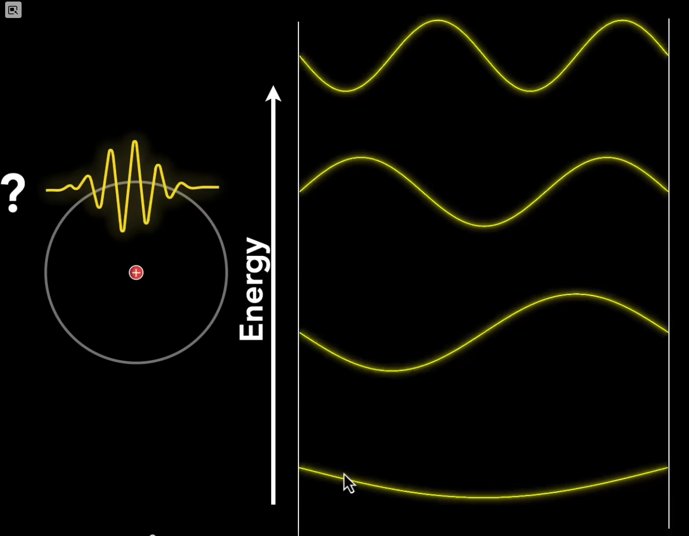
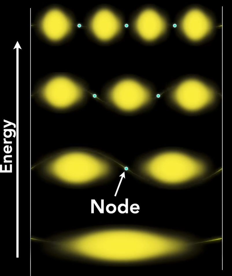
-
And arrive at this 3D visualization:
-
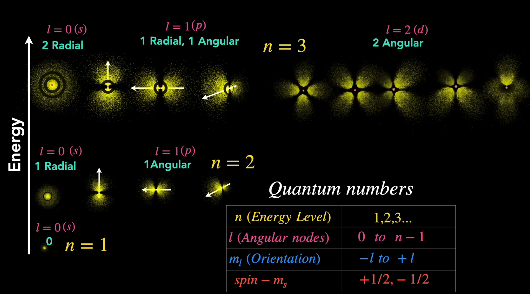 .
.
-
All the visual characteristics of the visualization come from the ways in which the nodes can be represented.
-
Apparently nodes can be radial or angular. The angular representations appear when considering that the node can be a plane.
-
It is these nodes represented as a plane that make the shapes more interesting.
-
-
The "overlap" I mentioned is not about spatial overlap. It's about mathematical independence.
-
Spherical harmonics are precisely the spherical analogue of the Fourier transform.
-
Fourier Series (for a function on a circle): Any function on a 1D circle (like a sound wave over time) can be broken down into a sum of simple, orthogonal basis functions: sines and cosines of different frequencies (
sin(nθ),cos(nθ)).-
The low-frequency sines/cosines capture the broad, smooth shape.
-
The high-frequency ones capture the sharp details and edges.
-
-
Spherical Harmonics (for a function on a sphere): Any function on a 2D sphere (like an environment map) can be broken down into a sum of simple, orthogonal basis functions: the spherical harmonics (
Y_lm(θ, φ)).-
The low-
l(low-frequency) SHs capture the broad, smooth lighting (the average color, the dominant light direction). -
The high-
l(high-frequency) SHs capture the sharp details and edges (sharp reflections, tiny light sources).
-
-
We are not projecting a 3D scene onto a sphere.
-
This is called environment map capture (e.g., taking a 360° photo). That gives us a function
f(θ, φ)that is defined on the surface of a sphere.
-
-
The Spherical Harmonic transform is the next step. We are taking that already-spherical function
f(θ, φ)and projecting it onto the spherical harmonic basis functions. -
The word "projection" here is used in the linear algebra sense, just like projecting a vector onto a set of basis axes.
-
Imagine your environment map
f(ω)is a vector in a giant, infinite-dimensional space. -
The spherical harmonics
Ylm(ω)form a complete set of orthonormal basis vectors for that space. -
Projecting
fonto a specific basis vectorYlmis how we find the coefficientclmfor that function. The formula for this projection is the inner product:c_lm = ∫ f(ω) * Y_lm(ω) dω. -
This is identical to how in 3D space, you find the
x-component of a vectorVby projecting it onto the unitX basis vector:V_x = V • unitX. -
"Orthonormalization" means we have ensured two things for our basis functions
Y_lm:-
Orthogonal:
∫ Y_lm(ω) * Y_l'm'(ω) dω = 0if(l, m) ≠ (l', m')(they are independent). -
Normalized:
∫ Y_lm(ω) * Y_lm(ω) dω = 1(each one has a "unit length").
-
-
This orthonormality is what makes the math so clean and the coefficients independent.
-
In Quantum Mechanics, the spherical harmonics
Y_lmare famous because they are the angular solutions to the Laplace equation in spherical coordinates. -
This describes the probability distribution of an electron around a hydrogen atom (its orbital). The shapes of the s, p, d, f orbitals are visualizations of the
Y_lmfunctions!-
Y00is the s-orbital (spherical). -
Y1mare the three p-orbitals (dumbbell shaped along x, y, z). -
Y2mare the five d-orbitals (cloverleaf shapes).
-
-
In Computer Graphics: We are using the exact same mathematical functions to describe the distribution of light energy around a point. The "orbital" is now the "irradiance environment."
-
The key difference is one of interpretation:
-
In Quantum Mechanics, you're solving for a wavefunction.
-
In Computer Graphics, you're using the SH basis to compactly represent a function (light) defined on a sphere.
-
The process for computer graphics :
-
For a render engineer, the process is this:
-
Capture/Define: Start with an environment map
f(ω). This is your function on the sphere. -
Project (Precompute/Integrate): For each SH basis function
Y_lmyou care about (e.g., the first 9), compute the coefficientc_lmby integrating the productf(ω) * Y_lm(ω)over the entire sphere. This is the "transformation" into the SH frequency space.c_lm = ∫ f(ω) * Y_lm(ω) dω -
Reconstruct (Runtime): To get the approximate value of the environment at any direction
ω, you evaluate the sum:f(ω) ≈ Σ c_lm * Y_lm(ω)forl=0...N-1.
-
-
The reason this is a "convolution" is that the rendering equation often includes a cosine term (
n • ω). The magic is that projecting this cosine lobe into SH space results in analytic attenuation factors (A_l) that you can just multiply by yourc_lmcoefficients before the reconstruction step. This turns a complex integral into a simple dot product of two SH vectors (lighting coefficients and attenuated coefficients). -
So, you were right on all counts. It is a Fourier-style transform. It is a projection onto an orthonormal basis. And it uses the same elegant math as quantum physics to solve a seemingly unrelated problem in computer graphics with breathtaking efficiency.
-
Application :
-
Spherical Harmonics Exponentials for Efficient Glossy Reflections .
-
I watched a bit of the video, very technical and specific, about an optimization for computing glossiness.
-
 .
.
-
Ringing happens when you try using high order spherical harmonics.
-
-
-
Solutions
ReSTIR GI
-
ReSTIR GI is a spatio-temporal resampling algorithm for path/path-sample reuse (improving sampling of indirect lighting), i.e., a sampling/resampling approach for path/path-trace-based GI rather than a probe or voxel store.
-
Kajiya .
Lumen
-
-
We settled on Mesh Signed Distance Fields for our Software Ray Tracing geometry representation. These give reliable occlusion, all areas have coverage, and we still get fast software ray tracing through sphere tracing, which skips through empty space. The intersection with the distance field surface only gives us the hit position and normal, we can’t find the material attributes or the lighting.
-
We tried runtime voxelization and voxel cone tracing, but merging geometry properties into a volume causes lots of leaking, especially in the lower mip maps.
-
We also tried voxel bit bricks, where we stored 1 bit per voxel to mark whether it contains geometry or not. Simple ray marching of bit bricks was surprisingly slow and after adding a proximity map for acceleration, we just decided to drop voxels and arrived at a Global Distance Field
-
-
Radiance Caching for Real-time Global Illumination - 2021 .
-
I watched the first 10 minutes of the video.
-
-
Keywords:
-
Downsample incoming radiance.
-
-
-
Probes:
-
Octahedral atlas with border.
-
8x8 per probe, resulting in 64 traces per probe.
-
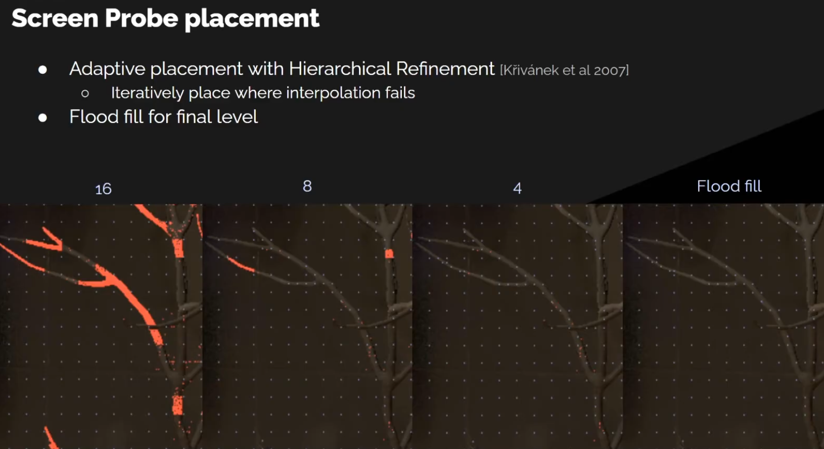 .
.
-
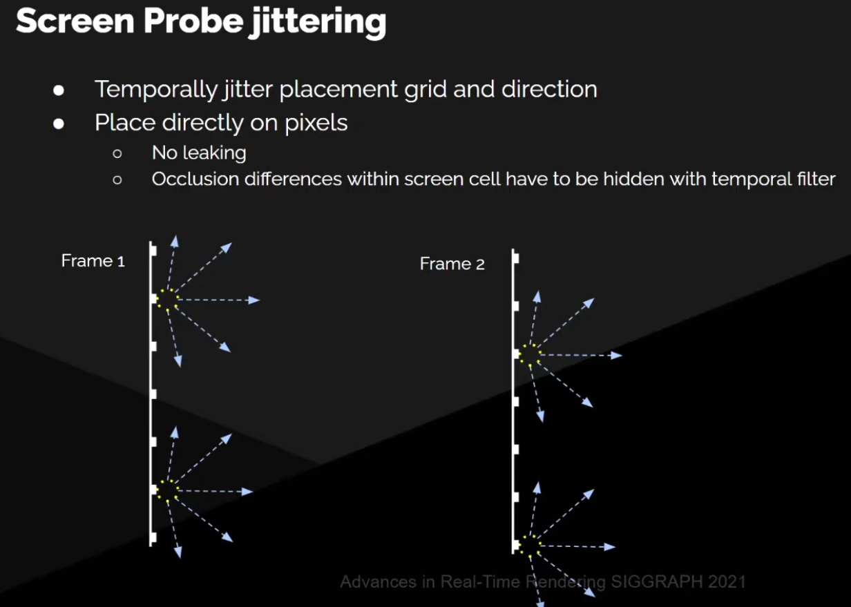 .
.
-
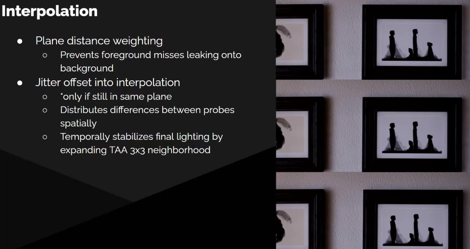 .
.
-
Screen Space Radiance Caching
-
-
UE5 - Instead of tracing for every single pixel on screen, we bundle up our rays and we trace from a much smaller set of pixels.
-
Two-Level Radiance Caching - AMD - GDC 2023 .
-
Instead tradeoff between pathtracing and probes.
-
Less noise with less samples, sounds like a good idea.
-
-
-
SDF Rays.
-
Spatial Cascaded Cache.
-
Froxel Volumes.
-
Etc.
-
Intense.
-
I don't know if it is Forward+ or Deferred Rendering...
-
Radiance Cascades (RC)
-
Radiance Cascades: A Novel Approach to Calculating Global Illumination - August 2023 .
-
Implementation of Radiance Cascades in World Space, purely .
-
3D Demo .
-
-
A rendergraph-based graphical framework for Vulkan, in C++.
-
The author of Radiance Cascades contributed to this engine.
-
Radiance Cascades is not implemented in this engine.
-
-
They require a lot of compute and memory in 3D space.
-
For 2D and screen-space 3D (like in Path of Exile 2) the amount of data you store is small enough that RC is an efficient solution, but it doesn't scale well for large 3D worlds.
-
Path of Exile 2.
-
Godot Discussion:
-
Juan (against):
-
Despite the hype, radiance cascades actually aren't all that practical, or at least aren't any more practical than competing techniques, in world space mode.
-
Radiance cascades shine in screen space mode (which is why they work excellently for Path of Exile), so they're less an alternative to Lumen/SDFGI and more an alternative to SSGI.
-
-
fakhraldin (in favor):
-
Suggested Radiance Cascades.
-
This GI solution is not restricted to 2D. Why should a probe based GI be restricted to only 2D in the first place? This doesn't make any sense for every graphics developer who got experience with probe based GI techniques, strange.
-
Radiance Cascades are not restricted to screen space but can be expanded to polygonal hardware ray tracing as well. Alexander clearly confirms this here . And again it is strange to claim the opposite to every experienced graphics developer. In fact there are several released triple A titles, which use probe based GI with polygonal hardware ray tracing instead of screen space.
-
Screen Space is still being used even by triple A studios. Even Software Lumen itself does partially use SSGI for details of close objects among other techniques. Remember, Lumen is composed of several GI techniques. Million dollar game productions do rely on Screen Space. You don't come around using screen space for high frequency details in cross-gen graphics. Signed distance fields and voxel solutions are missing high frequency details.
-
-
Other people against:
-
We both very explicitly say that yes, radiance cascades can be used in world space. Their limitations just don't make them a better or more practical alternative to SDFGI/HDDAGI. We both very explicitly say that radiance cascades could be a great alternative to SSGI.
-
I would like to see someone create a 3D radiance cascades solution (open-world would be even better). I'm a bit skeptical about its performance since, even in screen space, it's not that impressive compared to other screen space solutions, though it does look better.
-
Juan stated in his thread, open-world is actually radiance cascade's greatest weakness as a world space effect.
-
This is actually what makes radiance cascades (as a screen space effect) really good and why it's used in production in Path of Exile: the cost is the same as other SSGI approaches, but the quality is much higher.
-
-
Neither SDFGI nor HDDAGI are proven as practical solutions. SDFGI is being replaced by HDDAGI due to its inefficacy, and HDDAGI isn't released yet. Neither have effective parity with production-proven GI techniques and are ultimately experimental.
-
Take Avatar Frontiers of Pandora for example. Their technique is currently seen as the most sophisticated dynamic GI solution for cross-gen and next-gen realtime video games.
-
But it may surprise many people that their solution actually shares a similar ground concept of "radiance cascades". They also use a probe based system. Instead of using radiance cascades, they combine different techniques like world space, screen space for high frequency details and ray tracing per hardware RT or compute shaders RT as a fallback. Similar to radiance cascades they implement additional different layers to achieve a wider spectrum of GI. They capture the world's details by "different grades of detection" so to speak.
-
The solution with "radiance cascades" is way less complicated, more performant and more scalable for hardware. Just like with SDFGI and HDDAGI we already use a probe grid. "Radiance Cascades" is just adding hierarchical probe grids with different resolutions to the existing one. This step increases detail capture and quality tremendously at cheap costs even with ray tracing.
-
We don't even need to make additional probe grids mandatory. It could be optional in the editor and even be offered as an in-game option. The more grid levels you can add, the more quality you can achieve according to your liking and machine. It is highly flexible.
-
From a technical standpoint i really don't see insurmountable objections against this solution, as it doesn't even interfere dramatically with the existing one. Rather it can serve as an additional, supportive and optional layer to the basic probe grid. If you don't want to apply it for world space, than don't do it. There are many another ways.
-
"Radiance Cascades" can be combined with world space and hardware rt or compute shaders rt to achieve similar results to ubisoft's GI solution, if not even better. Many features in godot turned out to be short-lived obsolete code. But i really don't see "Radiance Cascades" as such. It rather could serve as a basis for further development and options, which build upon it.
-
Our resources are limited and it would truly be a missed opportunity not to take advantage of this low-hanging fruit from which a great tree could grow.
-
World space radiance cascades has occlusion challenges (sound familiar?) and memory consumption challenges - just like pretty much all real time GI solutions.
-
However due to the specific nature of these challenges for radiance cascades, any practical implementation of world space radiance cascades will be limited to 3, at most 4, cascades.
-
What if you need GI for an open world map, for example? You might be able to make it work beyond that range, but most potential approaches are challenging to implement, and will likely be expensive to run.
-
For example, one potential approach is a cascade of radiance cascades. Literally running the entire thing multiple times at multiple sizes, and interpolating between them.
-
So, you might say: "well maybe it can just be a higher quality short range alternative to SDFGI/HDDAGI?" You may have some misconceptions about the level of quality of world space radiance cascades, compared to its much more impressive screen space counterpart.
-
Watch this video that Sannikov himself posted . Does the blockiness and crawliness of the lighting look familiar to you? Does the volume representation look familiar to you? The quality tradeoffs of world space radiance cascades are very similar to the quality tradeoffs of SDFGI/HDDAGI. By replacing SDFGI/HDDAGI with world space radiance cascades, you are literally swapping it out with a technique that has practically the same quality, but much more limited range. You're gaining nothing, and losing something.
-
For screen space radiance cascades however, that's a different story. Pretty much everyone agrees it's incredible - probably the best screen space GI the industry has to offer right now, both in terms of performance and quality.
-
Author of Radiance Cascades, commenting on the HDDAGI PR:
-
First, I never pitched 3d RC as the ultimate GI solution. I never even pitched it as a good GI solution. I wouldn't even call it practically viable by my standards, to be honest. I'm just saying that it's a direct improvement (in pretty much all parameters) over anything that has a regular grid (or nested grids) of radiance probes. DDGI for example.
-
Second, the screenspace version of RC is only limited to on-screen occluders and light sources if screenspace raymarching is used. However, screenspace cascades can store worldspace radiance intervals (including offscreen geometry) if you have a way of casting worldspace rays, using either a BVH, an SDM or a voxel raymarcher of some sort. The main limitation of this approach is that it only allows storing radiance on the surface of the depth buffer and you can't use it for example for volumetric lighting.
-
-
Juan apparently thought of an approach that's even better than HDDAGI, and will eventually work on that instead of continuing HDDAGI.
-
Dynamic Diffuse Global Illumination (DDGI) / Ray-Traced Irradiance Fields
-
"Dynamic Diffuse Global Illumination with Ray-Traced Irradiance Fields" - Majercik 2019 .
-
Dynamic Diffuse Global Illumination with Ray-Traced Irradiance Fields - Majercik 2019 .
-
Much of the talk is about:
-
Fixing very common light leaks in techniques involving light probes.
-
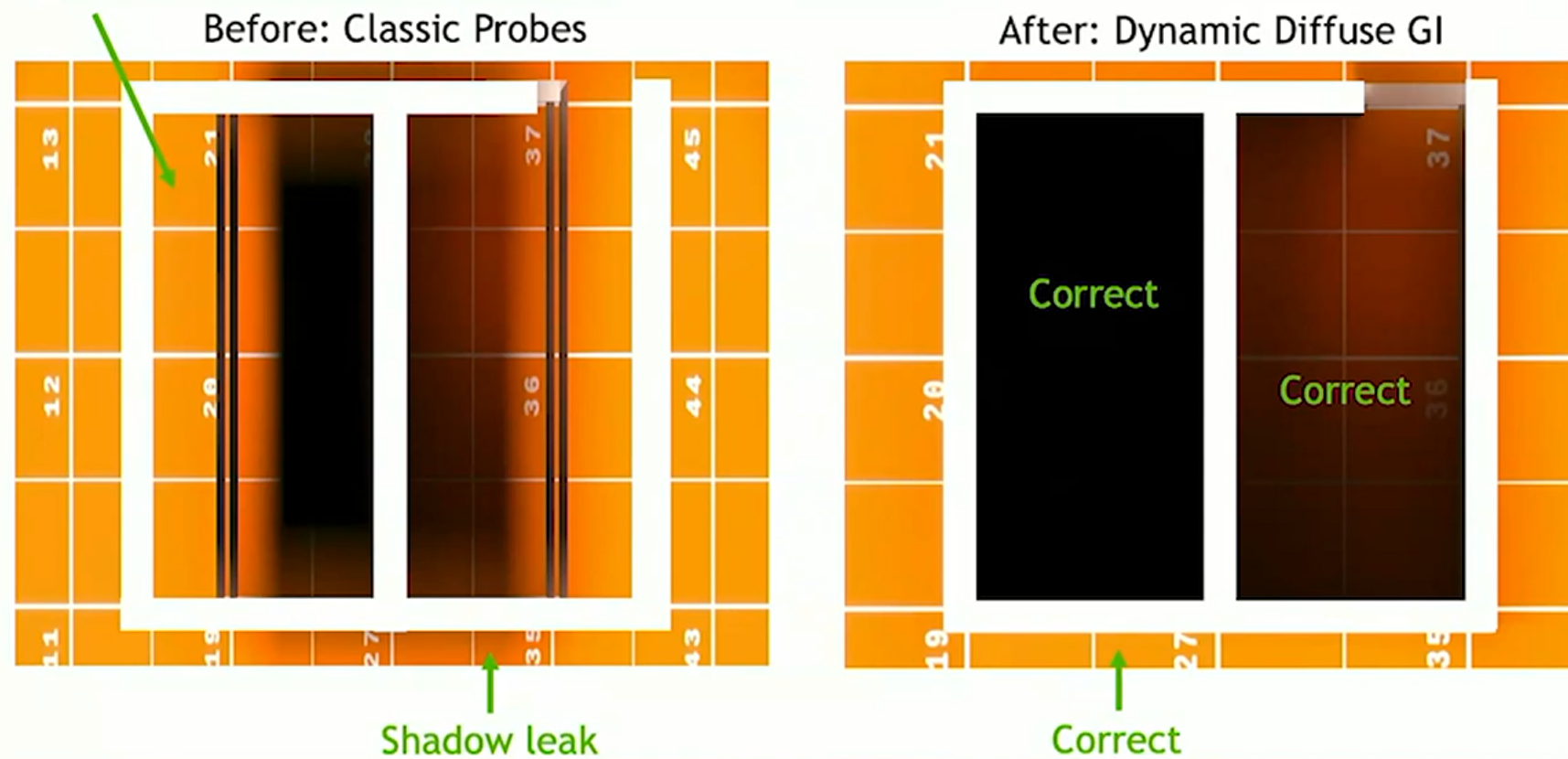 .
.
-
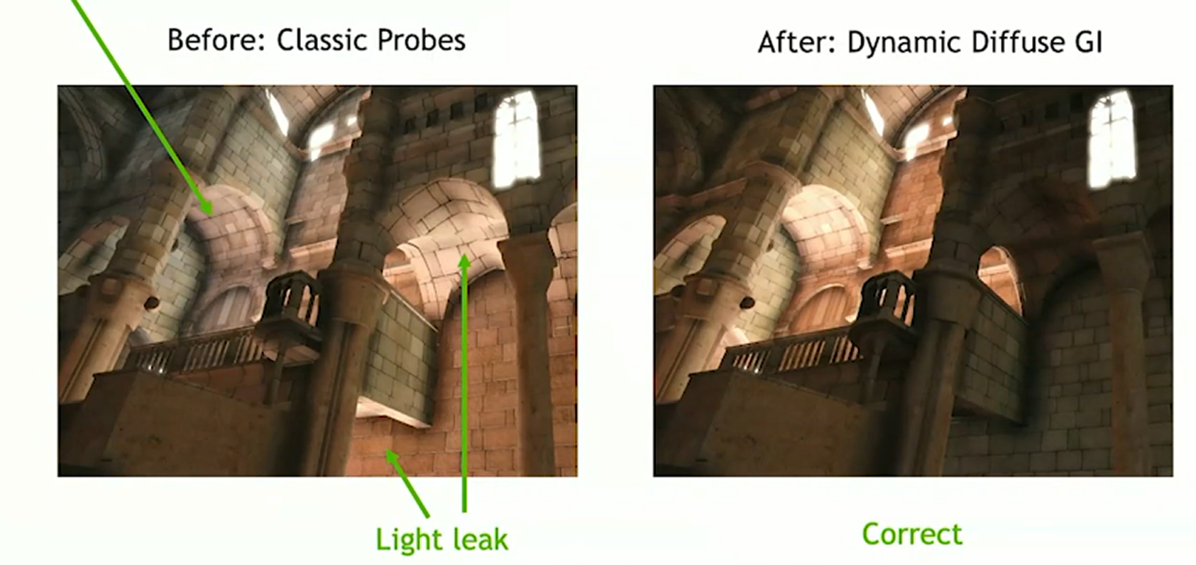 .
.
-
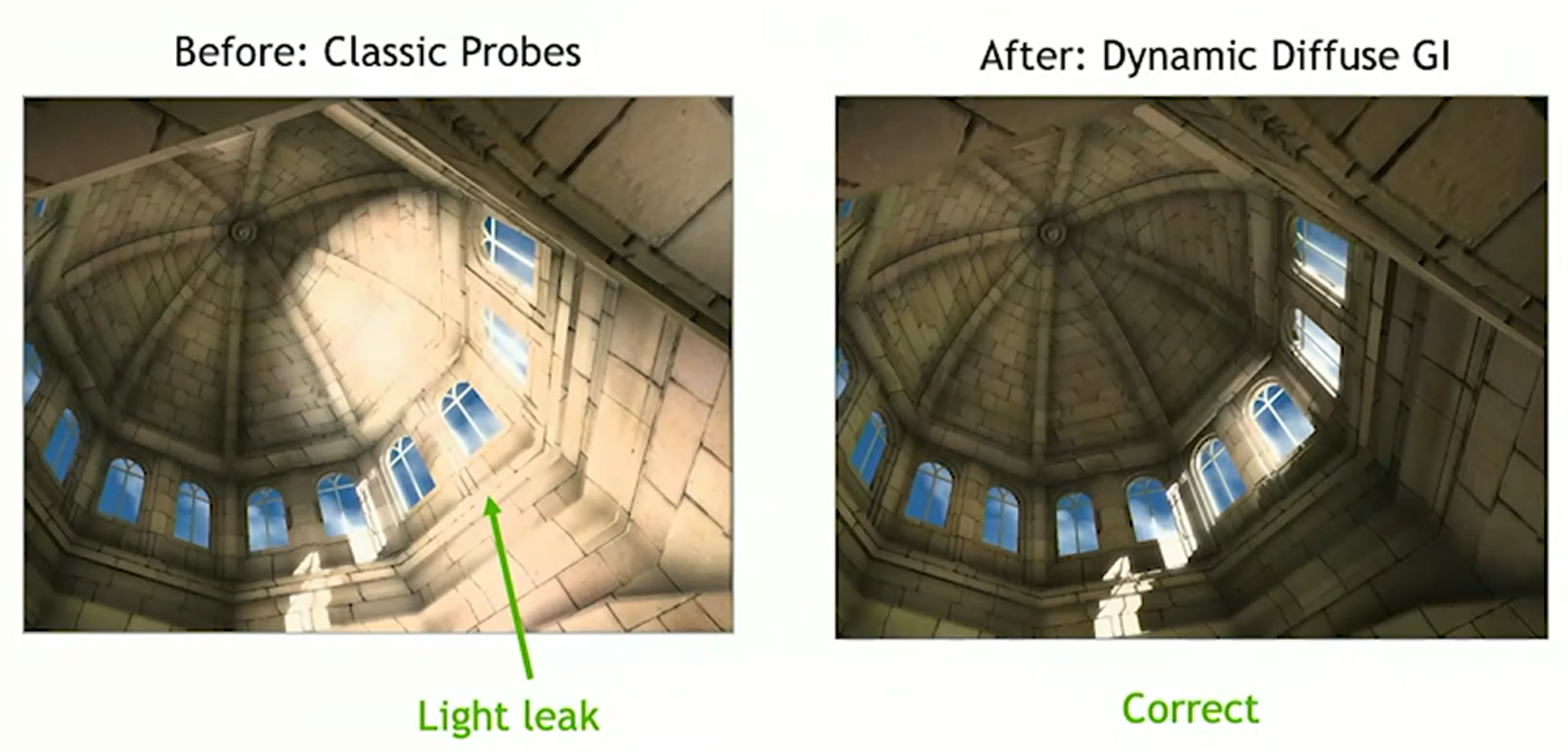 .
.
-
-
Better automatic placing of Light Probes.
-
-
"Up to 256 rays per probe per frame, scaled down in some cases".
-
Limitations :
-
Don't sample on the surface, as it's really unstable.
-
1mm up and you are ok, 1mm down and you are inside the surface, where everything is black.
-
Use a bias to improve this.
-
-
-
-
"Dynamic Diffuse Global Illumination with Ray-Traced Irradiance Fields" - Majercik 2019 .
-
"Scaling Probe-Based Real-Time Dynamic Global Illumination for Production" - Majercik 2021 .
-
"Improving Probes in Dynamic Diffuse Global Illumination" - Rohacek 2022 .
-
DDGI isn't an alternative to RTXGI, but a way to implement it using light probes.
-
Probes :
-
Uses probe volumes (a set of points in space storing irradiance + visibility).
-
A probe typically holds an estimate of irradiance or sometimes radiance distribution directly (often SH coefficients).
-
Comparing to PRT, the DDGI Probes represent the current lighting, not a precomputed transfer.
-
PRT probe = precomputed transfer.
-
“This is how light at this spot responds to any lighting, given the static scene geometry.”
-
-
DDGI probe = runtime-sampled irradiance.
-
“This is the actual indirect lighting at this spot right now, given whatever is in the scene.”
-
-
-
Probes store the incoming light in every single direction for rays passing through their center.
-
It may also store depth/visibility information (to reduce light leakage).
-
Each probe gathers lighting from the environment using ray tracing (usually hardware-accelerated).
-
Lighting between probes is interpolated at runtime.
-
When shading a point on a surface we sample the probes that are nearby, and blend for smooth lighting.
-
-
Requires a set of probes, each storing low-frequency irradiance (spherical harmonics, octahedral maps, or similar).
-
Probes can be updated progressively with ray tracing, amortizing cost across frames.
-
Usually only practical for low-frequency GI (no fine detail).
-
Bias samples for probes that just had changes in irradiance, like importance sampling, could speed convergence after edits.
Screen Space Indirect Lighting with Visibility Bitmask (VBAO) (SSILVB)
-
The technique is essentially an extension to ground-truth ambient occlusion (GTAO).
-
Huge performance gain from GTAO.
-
Quality visuals of near raytracing ambient occlusion.
-
Screen Space Indirect Lighting with Visibility Bitmask - 2023 .
-
SSAO vs GTAO vs SSILVB and implementation of SSILVB .
-
I didn't read it properly.
-
The implementation is adapted from "Screen Space Indirect Lighting with Visibility Bitmask" by Olivier Therrien https://cdrinmatane.github.io/posts/cgspotlight-slides/.
-
Horizon-Based Indirect Lighting
-
Horizon-Based Indirect Lighting - Benoit Patapom Mayoux 2018 .
-
"The ideal companion for your far-field indirect lighting solution".
-
Treat the depth buffer as sort of a height field and march across that in slices.
-
A horizon tells if new samples are hidden behind old samples.
-
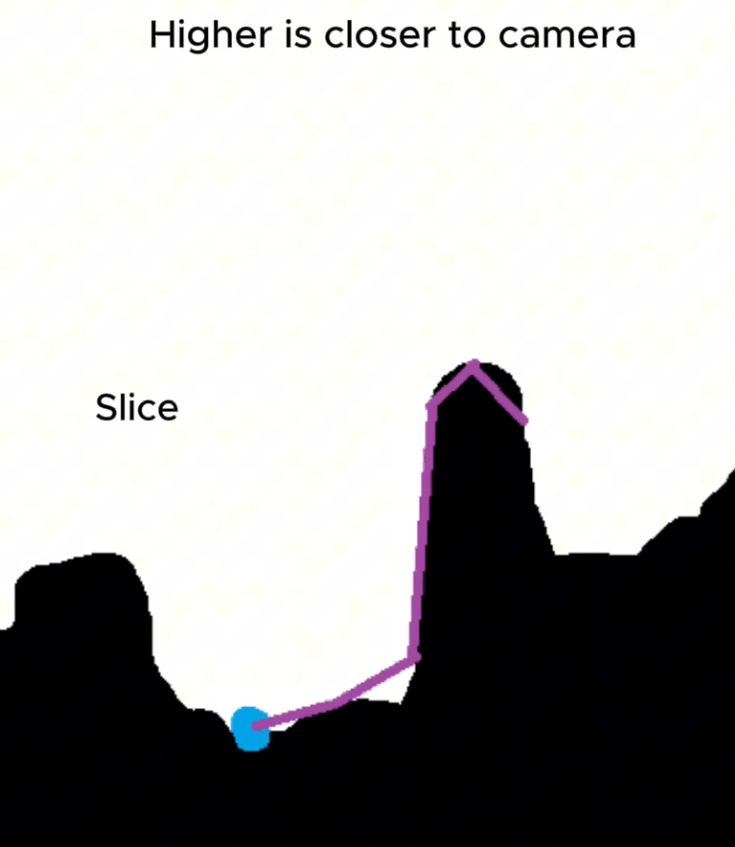
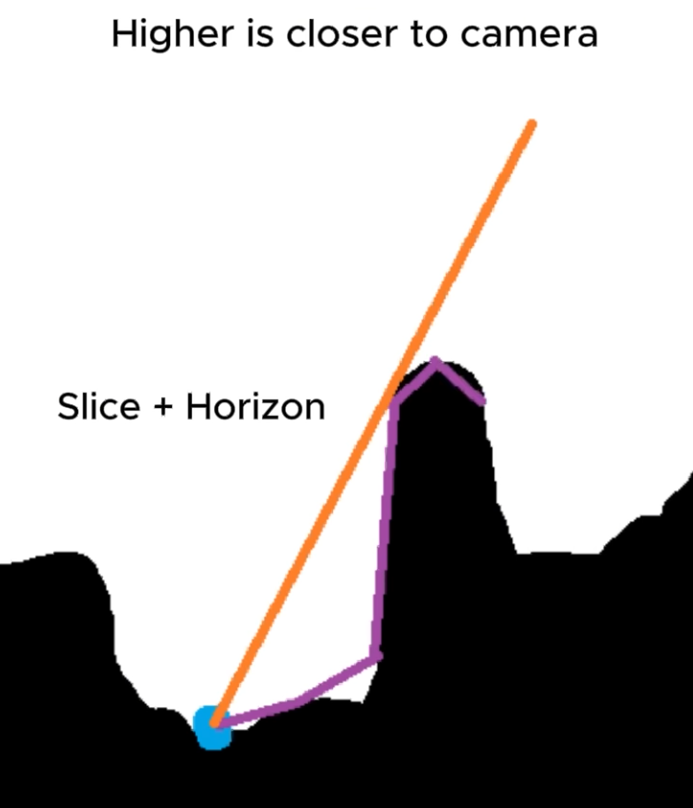 .
.
Multi-Scale Ambient Occlusion (MSAO)
-
Efficient screen-space approach to high-quality multiscale ambient occlusion - 2012
-
"I know HBAO+ is released but this method is far cheaper as you can see on that table in the end of the paper (They tested on GTX 460M! and it is 23ms average). I believe this method will give us far superior visuals than just SSAO."
-
Wicked Engine 2024 :
-
This was my favourite SSAO so far because it handles large areas and small detail alike without any noise or temporal issues. It works by computing the AO in a deinterleaved version of the depth buffer that is contained in a Texture2DArray. It computes the AO in multiple resolutions, then upsamples and combines all of them into a final texture with bilateral blurring.
-
Screen Space Reflection (SSR)
-
Used to capture reflections based on the rendered scene (using the previous frame for instance) by ray-marching in the depth buffer.
-
SSR gives great results but can be very expensive .
-
SSR - Wicked Engine 2017 Demo .
-
I implemented screen space reflections around two years ago but never showed it off so here you go.
-
This is the simplest technique that I know of. It is using binary search when raymarching in view space.
-
Distant Environment Probes / Cube Map IBL
-
Lightmaps, Ambient Color, IBL with CubeMaps, Probe-based Lighting .
-
Used to capture lighting information at “infinity”, where parallax can be ignored. Distant probes typically contain the sky, distant landscape features or buildings, etc.
-
The light is assumed to come from infinitely far away (which means every point on the object's surface uses the same environment map).
-
They are either captured by the engine or acquired from a camera as high dynamic range images (HDRI).
-
Irradiance :
-
The whole environment contributes light to a given point on the object's surface.
-
-
Radiance :
-
The resulting light bouncing off of the object.
-
-
Incident lighting must be applied consistently to the diffuse and specular parts of the BRDF.
-
Typically, the environment image is acquired offline in the real world, or generated by the engine either offline or at run time; either way, local or distant probes are used.
-
Obviously the environment image must be acquired somehow and as we'll see below it needs to be pre-processed before it can be used for lighting.
-
 .
.
-
Limitations :
-
Implementing a fully dynamic day/night cycle requires for instance to recompute the distant light probes dynamically.
-
As probes only capture basic color information and direction, very shiny surfaces are not very doable.
-
 .
.
-
Far Cry 3 used probes. In that game you wouldn't find any shiny metallic object, as the probes cannot represent that type of lighting very easily.
-
IBL Cube Maps, on the other hand, could represent metals much better.
-
 .
.
-
Images, in particular cubemaps, are a great way to encode such an “environment light”.
-
-
Processing Light Probes :
-
We saw previously that the radiance of an IBL is computed by integrating over the surface's hemisphere.
-
Since this would obviously be too expensive to do in real-time, we must first pre-process our light probes to convert them into a format better suited for real-time interactions.
-
The sections below will discuss the techniques used to accelerate the evaluation of light probes:
-
Specular reflectance :
-
pre-filtered importance sampling and split-sum approximation
-
-
Diffuse reflectance :
-
irradiance map and spherical harmonics
-
-
-
-
Implementation (Filament) :
vec3 irradianceSH(vec3 n) { // uniform vec3 sphericalHarmonics[9] // We can use only the first 2 bands for better performance return sphericalHarmonics[0] + sphericalHarmonics[1] * (n.y) + sphericalHarmonics[2] * (n.z) + sphericalHarmonics[3] * (n.x) + sphericalHarmonics[4] * (n.y * n.x) + sphericalHarmonics[5] * (n.y * n.z) + sphericalHarmonics[6] * (3.0 * n.z * n.z - 1.0) + sphericalHarmonics[7] * (n.z * n.x) + sphericalHarmonics[8] * (n.x * n.x - n.y * n.y); } // NOTE: this is the DFG LUT implementation of the function above vec2 prefilteredDFG_LUT(float coord, float NoV) { // coord = sqrt(roughness), which is the mapping used by the // IBL prefiltering code when computing the mipmaps return textureLod(dfgLut, vec2(NoV, coord), 0.0).rg; } vec3 evaluateSpecularIBL(vec3 r, float perceptualRoughness) { // This assumes a 256x256 cubemap, with 9 mip levels float lod = 8.0 * perceptualRoughness; // decodeEnvironmentMap() either decodes RGBM or is a no-op if the // cubemap is stored in a float texture return decodeEnvironmentMap(textureCubeLodEXT(environmentMap, r, lod)); } vec3 evaluateIBL(vec3 n, vec3 v, vec3 diffuseColor, vec3 f0, vec3 f90, float perceptualRoughness) { float NoV = max(dot(n, v), 0.0); vec3 r = reflect(-v, n); // Specular indirect vec3 indirectSpecular = evaluateSpecularIBL(r, perceptualRoughness); vec2 env = prefilteredDFG_LUT(perceptualRoughness, NoV); vec3 specularColor = f0 * env.x + f90 * env.y; // Diffuse indirect // We multiply by the Lambertian BRDF to compute radiance from irradiance // With the Disney BRDF we would have to remove the Fresnel term that // depends on NoL (it would be rolled into the SH). The Lambertian BRDF // can be baked directly in the SH to save a multiplication here vec3 indirectDiffuse = max(irradianceSH(n), 0.0) * Fd_Lambert(); // Indirect contribution return diffuseColor * indirectDiffuse + indirectSpecular * specularColor; } -
Implementation (Vulkan-glTF-PBR) :
-
The snippets below come from
material_pbr.frag
// Calculation of the lighting contribution from an optional Image Based Light source. // Precomputed Environment Maps are required uniform inputs and are computed as outlined in [1]. // See our README.md on Environment Maps [3] for additional discussion. vec3 getIBLContribution(PBRInfo pbrInputs, vec3 n, vec3 reflection) { float lod = (pbrInputs.perceptualRoughness * uboParams.prefilteredCubeMipLevels); // retrieve a scale and bias to F0. See [1], Figure 3 vec3 brdf = (texture(samplerBRDFLUT, vec2(pbrInputs.NdotV, 1.0 - pbrInputs.perceptualRoughness))).rgb; vec3 diffuseLight = SRGBtoLINEAR(tonemap(texture(samplerIrradiance, n))).rgb; vec3 specularLight = SRGBtoLINEAR(tonemap(textureLod(prefilteredMap, reflection, lod))).rgb; vec3 diffuse = diffuseLight * pbrInputs.diffuseColor; vec3 specular = specularLight * (pbrInputs.specularColor * brdf.x + brdf.y); // For presentation, this allows us to disable IBL terms // For presentation, this allows us to disable IBL terms diffuse *= uboParams.scaleIBLAmbient; specular *= uboParams.scaleIBLAmbient; return diffuse + specular; }-
Code where the IBL is calculated and used.
// Bla bla bla, basic lighting. vec3 F = specularReflection(pbrInputs); float G = geometricOcclusion(pbrInputs); float D = microfacetDistribution(pbrInputs); const vec3 u_LightColor = vec3(1.0); vec3 diffuseContrib = (1.0 - F) * diffuse(pbrInputs); vec3 specContrib = F * G * D / (4.0 * NdotL * NdotV); vec3 color = NdotL * u_LightColor * (diffuseContrib + specContrib); // Calculate lighting contribution from image based lighting source (IBL) color += getIBLContribution(pbrInputs, n, reflection); const float u_OcclusionStrength = 1.0f; // -> Ambient Occlusion // Apply optional PBR terms for additional (optional) shading if (material.occlusionTextureSet > -1) { float ao = texture(aoMap, (material.occlusionTextureSet == 0 ? inUV0 : inUV1)).r; color = mix(color, color * ao, u_OcclusionStrength); } // Emissive vec3 emissive = material.emissiveFactor.rgb * material.emissiveStrength; if (material.emissiveTextureSet > -1) { emissive *= SRGBtoLINEAR(texture(emissiveMap, material.emissiveTextureSet == 0 ? inUV0 : inUV1)).rgb; }; color += emissive; outColor = vec4(color, baseColor.a); -
Reflection Probes / Cube Map Reflections
-
Store environment radiance (not just irradiance ).
-
Stores a cube map texture of the surroundings, representing light incoming from all directions.
-
Usage :
-
Used for specular reflections (environment mapping).
-
Mipmapped cube maps can be used with roughness filtering (for PBR specular).
-
-
Good fits :
-
Games with a lot of metals, as that's where cube maps "shine" (literally).
-
Racing games are a good fit.
-
-
Limitations :
-
They are static; if the scene changes, the cubemap needs to be regenerated, and that's expensive.
-
Doesn't handle self-reflections.
-
 .
.
-
-
-
-
Reflection probes are used as a source of reflected and ambient light for objects inside their area of influence.
-
They can be used to provide more accurate reflections than VoxelGI and SDFGI while being fairly cheap on system resources.
-
Since reflection probes can also store ambient light, they can be used as a low-end alternative to VoxelGI and SDFGI when baked lightmaps aren't viable (e.g. in procedurally generated levels).
-
Good reflections, but poor indirect lighting.
-
Indirect lighting can be disabled, set to a constant color spread throughout the probe, or automatically read from the probe's environment (and applied as a cubemap). This essentially acts as local ambient lighting. Reflections and indirect lighting are blended with other nearby probes.
-
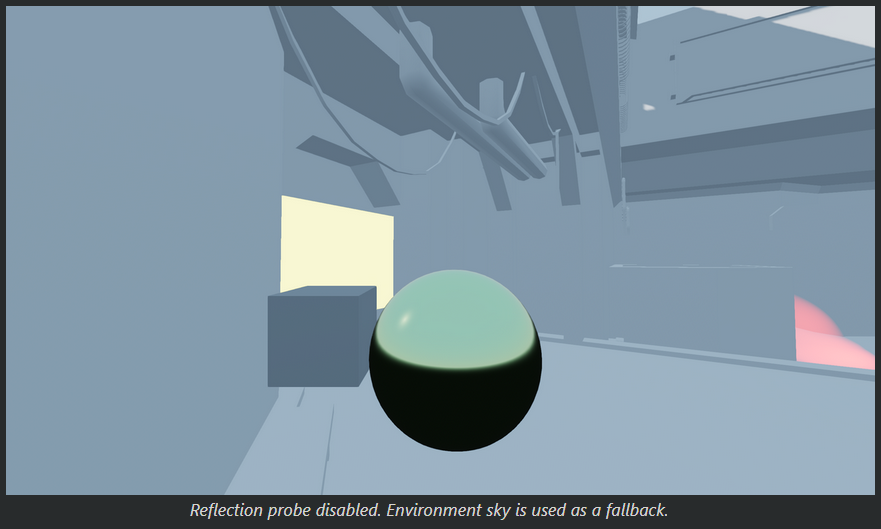
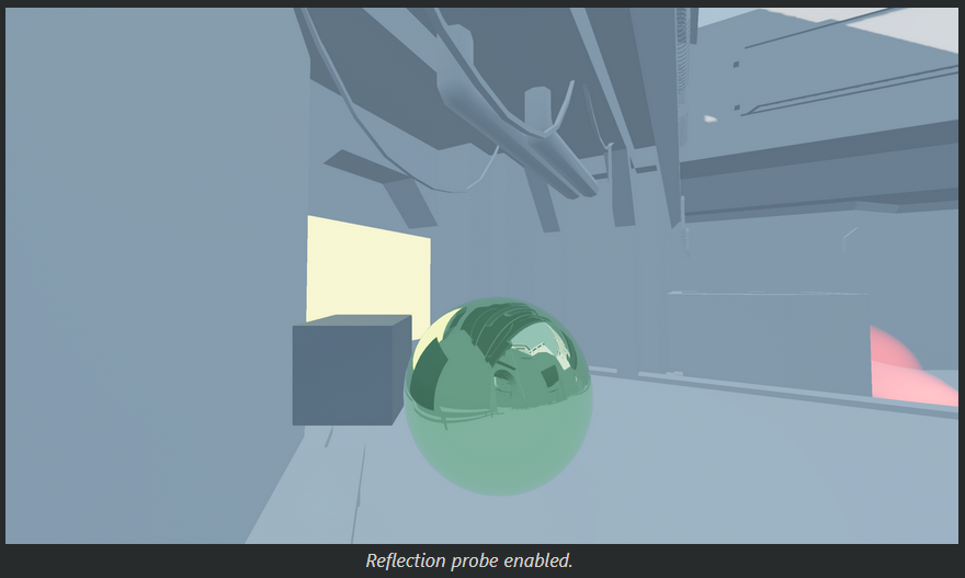 .
.
-
It interacts with LightmapGI:
-
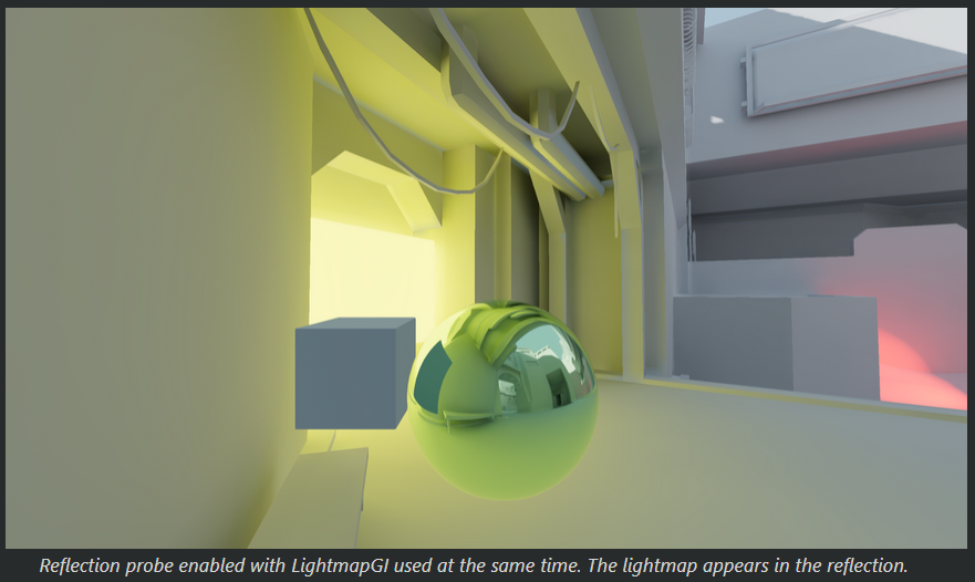 .
.
-
-
Reflection probes can also be used at the same time as SSR to provide reflections for off-screen objects.
-
Godot will blend together the SSRs and reflections from reflection probes.
-
This way you can get the best of both worlds: high-quality reflections for general room structure (that remain present when off-screen), while also having real-time reflections for small details.
-
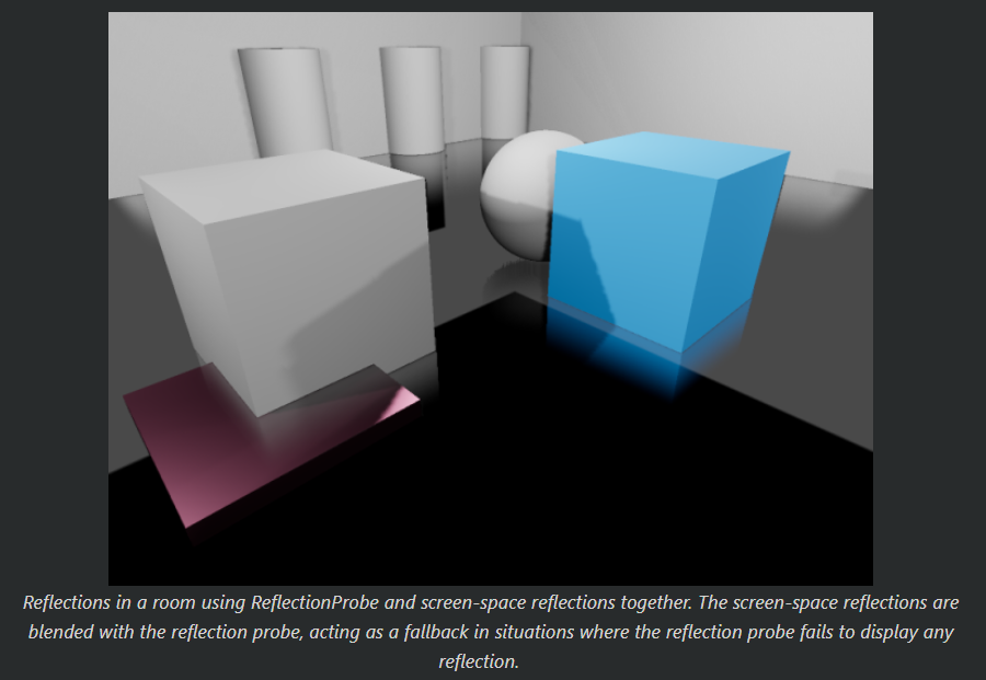 .
.
-
-
To get reasonably accurate reflections, you should generally have one ReflectionProbe node per room (sometimes more for large rooms).
-
The extents don't have to be square, and you can even rotate the ReflectionProbe node to fit rooms that aren't aligned with the X/Z grid.
-
Use this to your advantage to better cover rooms without having to place too many ReflectionProbe nodes.
-
-
Blending :
-
To make transitions between reflection sources smoother, Godot supports automatic probe blending:
-
Up to 4 ReflectionProbes can be blended together at a given location. A ReflectionProbe will also fade out smoothly back to environment lighting when it isn't touching any other ReflectionProbe node.
-
SDFGI and VoxelGI will blend in smoothly with ReflectionProbes if used. This allows placing ReflectionProbes strategically to get more accurate (or fully real-time) reflections where needed, while still having rough reflections available in the VoxelGI or SDFGI's area of influence.
-
-
To make several ReflectionProbes blend with each other, you need to have part of each ReflectionProbe overlap each other's area. The extents should only overlap as little as possible with other reflection probes to improve rendering performance (typically a few units in 3D space).
-
-
Performance :
-
ReflectionProbes with their update mode set to Always are much more expensive than probes with their update mode set to Once (the default). Suited for integrated graphics when using the Once update mode.
-
-
-
Rotate the camera 6 times to render the 6 faces of the cube.
-
You only render the plane, not the Tea Pot.
-
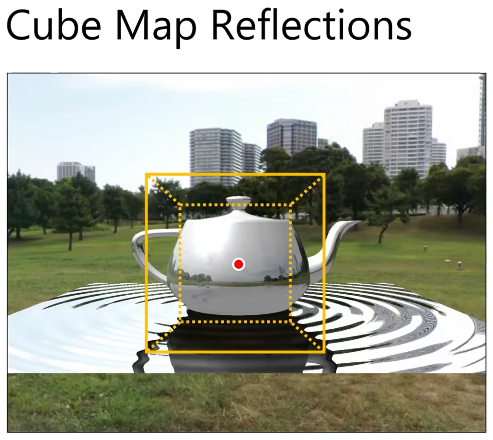
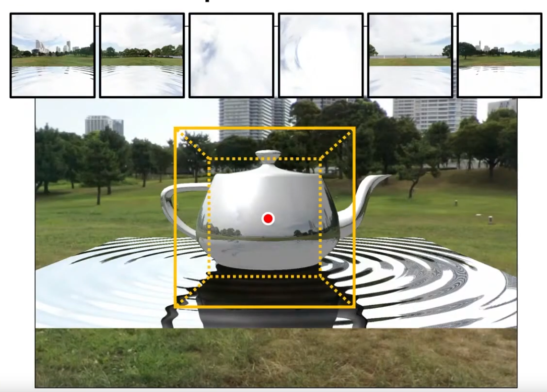 .
.
-
Instead of using the environment map loaded, you use the cubemap generated. So the reflection ON the Tea Pot only comes from this Cube Map.
-
You should also use the Cube Map on the mirror image of the Tea Pot (made when using Planar Reflections).
-
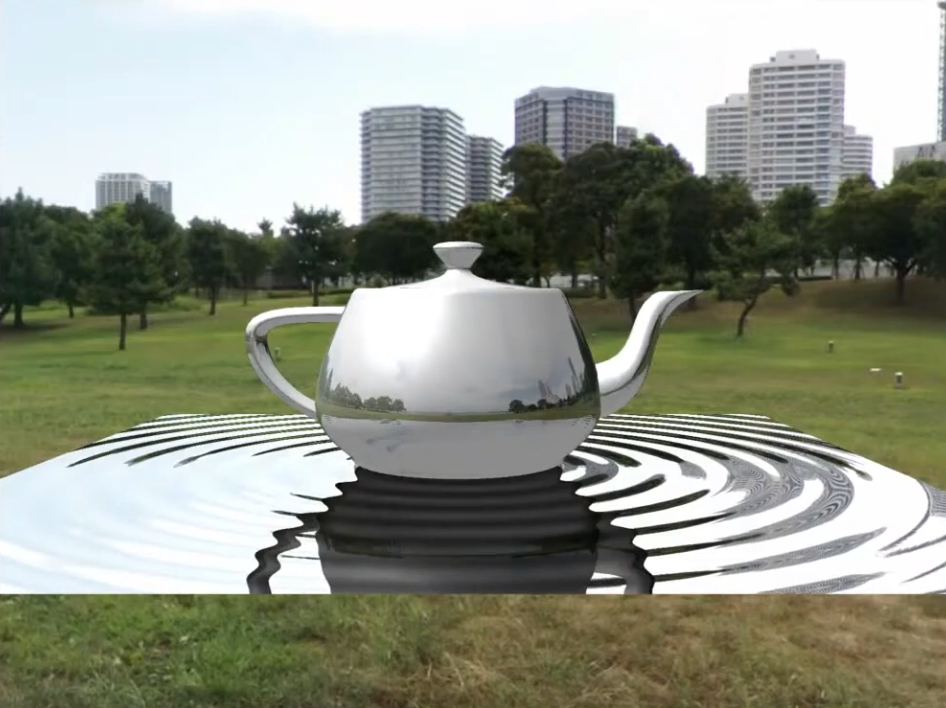 .
.
-
The mirror image is clearer now.
-
-
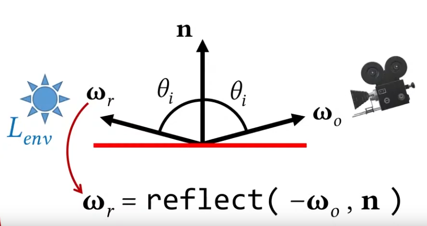 .
.
Planar Reflections / Flat Mirror
-
Used to capture reflections by rendering the scene mirrored by a plane. This technique works only for flat surfaces such as building floors, roads and water.
-
Instead of reflecting the entire world, we reflect the camera; it's the same thing.
-
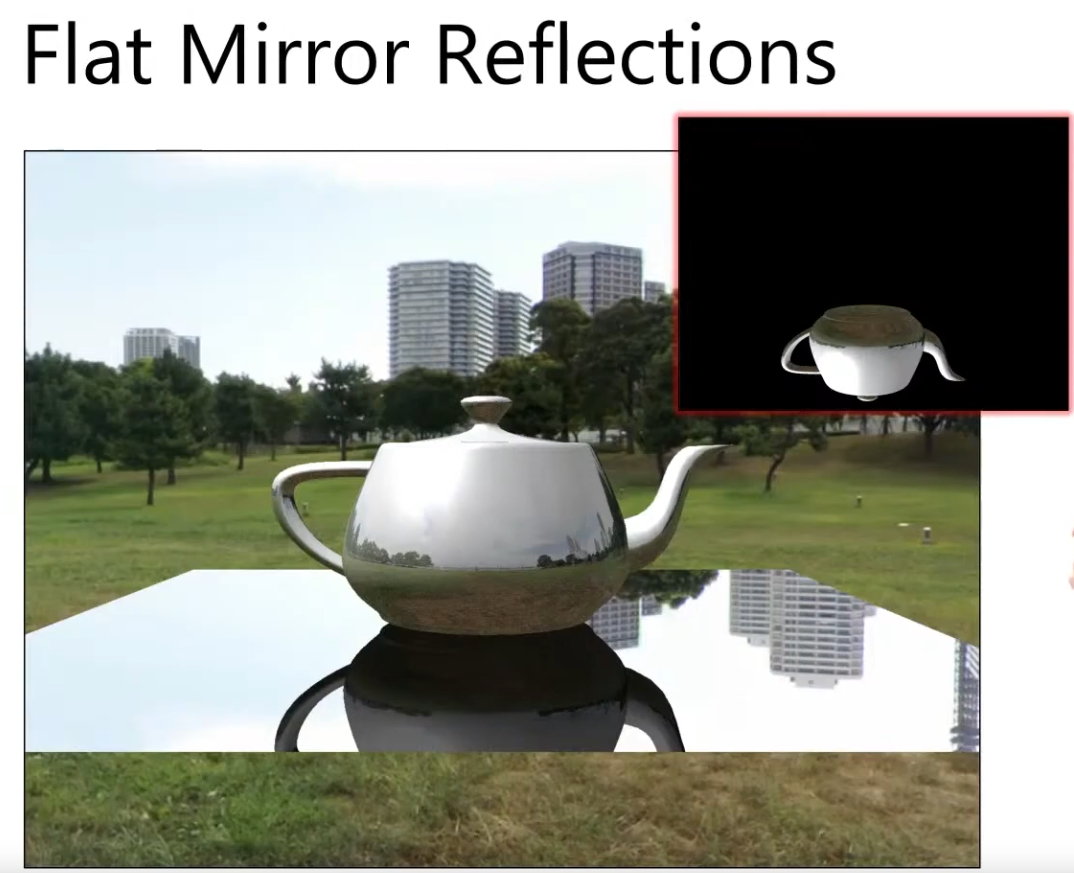 .
.
-
-
I’m disappointed whenever I see a modern game not supporting proper mirror reflections or if it has screen space reflection (SSR) on flat water. That’s why in Wicked Engine I’d like to show that planar reflection is still relevant and it should be one of the first choices of a game when a reflection needs to be rendered. The planar reflection is the perfect solution for a mirror because that’s what it was made for, and it’s good enough to use even on a large water surface with waves, like an ocean or a lake. Even though the waves are not totally accurate to be represented, it’s still a lot better than noisy SSR that cuts of abruptly.
-
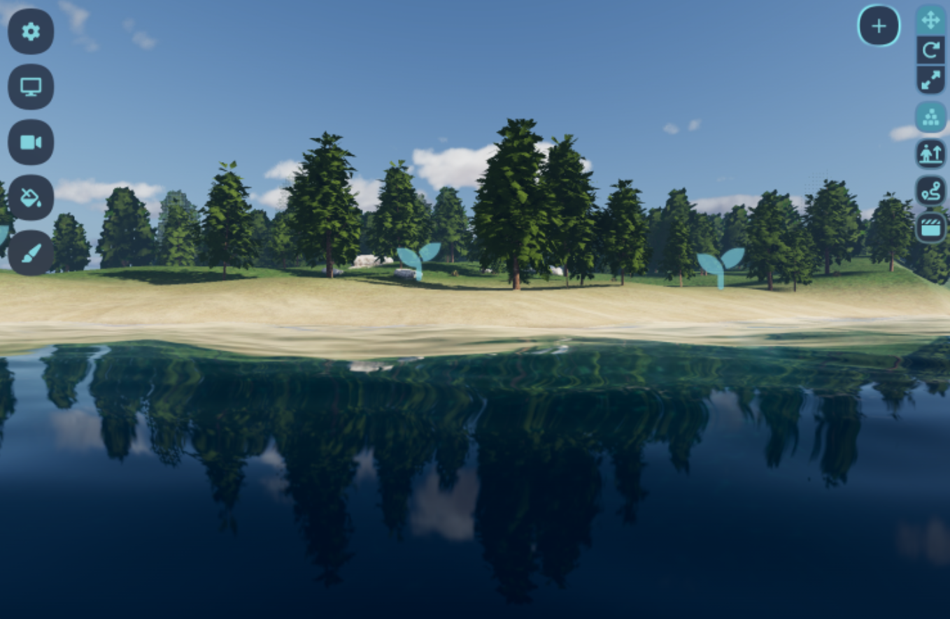 .
.
-
In Wicked Engine, the planar reflections are using a second full depth prepass + color pass with all the forward rendering pipeline capabilities. Although most of the secondary effects are turned off for them, simply by not running those passes for planar reflections. Also they don’t generate visibility buffer, only depth buffer in the prepass. Planar reflections rendering is also scheduled in the frame asynchronously to the main camera’s compute effects, so there is also room to utilize the modern graphics API to render them. Compared to the main camera, planar reflections are rendered in quarter of the main camera resolution in both axes so they become less dependent on the pixel shader performance, but more geometry heavy, which helps a bit with async compute passes at the same time. To combat the low resolution look, I choose to render them at 4x MSAA right now for some additional anti-aliasing. Quarter resolution means that the resolution is 1/16 compared to the main camera, and adding 4x MSAA on top doesn’t bring back the full detail, but I found it quite nice, for now, although it can be tweaked easily if needed.
-
Discarded Solutions
Voxel Cone Tracing GI (VCT) / Voxel GI / Sparse Voxel Octree GI (SVOGI) / Voxel Traced Global Illumination (VTGI)
-
Interactive Indirect Illumination Using Voxel Cone Tracing - 2011 .
-
Instead of using rays, we use voxel cones.
-
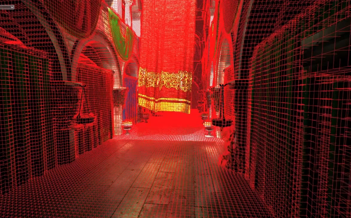 .
.
-
This is a high resolution of voxelization.
-
-
Just like mipmaps, we generate lower and lower resolutions of this.
-
And cones are used, where each cone accounts for a range of directions, instead of a single direction.
-
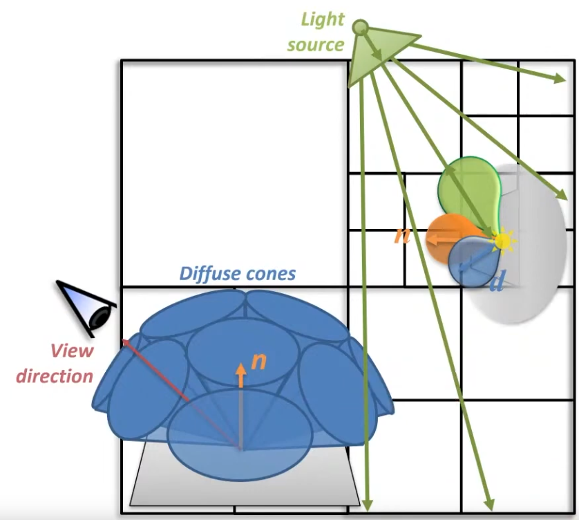 .
.
-
The cone tracing technique works best with a regular voxel grid because we perform ray-marching against the data like with screen space reflections for example.
-
A regular voxel grid consumes more memory, but it is faster to create (voxelize), and more cache efficient to traverse (ray-march).
-
The nice thing about this technique is that we can retrieve all sorts of effects. We have “free” ambient occlusion by default when doing this cone tracing, light bouncing, but we can retrieve reflections, refractions and shadows as well from this voxel structure with additional ray march steps. We can have a configurable amount of light bounces. Cone tracing code can be shared between the bouncing and querying shader and different types of rays as well. The entire thing remains fully on the GPU, the CPU is only responsible for command buffer generation.
-
Limitations / Drawbacks :
-
The main drawback being the limited resolution.
-
Voxel GI gives plausible multi-bounce GI but costs in memory, bandwidth and costly voxelization/update;
-
The UE5 presentation does make a good argument against cone tracing for generic use (which unreal engine targets), there will always be some artifacts and those will be super bad in specific scenes.
-
Comparing to RTGI, voxel based is faster but less accurate and less dynamic.
-
Voxel-based lighting is only faster than ray traced global illumination solutions that favor quality over performance. RTGI solutions that prioritize performance are faster than Voxel cone tracing.
-
Indiana Jones runs at 1080 60FPS on Series S with RTGI and KCD2 runs at 1080P 30 FPS on Series S.
-
Voxel cone tracing is an obsolete technological dead end - too heavy to run on last-gen consoles and mobile, inferior to RT on modern desktop and console hardware.
-
KCD2 (Kingdom Come: Deliverance II) only uses it because CryEngine supports it but doesn’t support ray tracing. And CryEngine is still stuck using voxel lighting because the Star Citizen devs poached CryTek’s best graphics engineers, and those engineers then proceeded to add ray tracing to Star Citizen’s fork of CryEngine.
-
SVOGI is inaccurate as balls.
-
You must love light leaking through every room corner. It's cheap crappy raytracing and it looks like cheap crappy raytracing.
-
-
Implementation :
-
First, we have our scene model with polygonal meshes. We need to convert it to a voxel representation. The voxel structure is a 3D texture which holds the direct illumination of the voxelized geometries in each pixel. There is an optional step here which I describe later. Once we have this, we can pre-integrate it by creating a mipmap chain for the resource. This is essential for cone tracing because we want to ray-march the texture with quadrilinear interpolation (sampling a 3D texture with min-mag-mip-linear filtering). We can then retrieve the bounced direct illumination in a final screen space cone tracing pass. The additional step in the middle is relevant if we want more bounces, because we can dispatch additional cone tracing compute shader passes for the whole structure (not in screen space).
-
1.) Voxelization :
-
The most involving part is definitely the first one, the voxelization step. It involves making use of advanced graphics API features like geometry shaders, abandoning the output merger and writing into resources “by hand”. We can also make use of new hardware features like conservative rasterization and rasterizer ordered views, but we will implement them in the shaders as well.
-
The main trick to be able to run this in real time is that we need to parallelize the process well. For that, we will exploit the fixed function rasterization hardware, and we will get a pixel shader invocation for each voxel which will be rendered. We also do only a single render pass for every object.
-
We need to integrate the following pipeline to our scene rendering algorithm:
-
1.) Vertex shader
-
The voxelizing vertex shader needs to transform vertices into world space and pass through the attributes to the geometry shader stage. Or just do a pass through and transform to world space in the GS, doesn’t matter.
-
2.) Geometry shader
-
This will be responsible to select the best facing axis of each triangle received from the vertex shader. This is important because we want to voxelize each triangle once, on the axis it is best visible, otherwise we would get seams and bad looking results.
// select the greatest component of the face normal input[3] is the input array of three vertices float3 facenormal = abs(input[0].nor + input[1].nor + input[2].nor); uint maxi = facenormal[1] > facenormal[0] ? 1 : 0; maxi = facenormal[2] > facenormal[maxi] ? 2 : maxi;-
After we determined the dominant axis, we need to project to it orthogonally by swizzling the position’s xyz components, then setting the z component to 1 and scaling it to clip space.
for (uint i = 0; i < 3; ++i) { // voxel space pos: output[i].pos = float4((input[i].pos.xyz - g_xWorld_VoxelRadianceDataCenter) / g_xWorld_VoxelRadianceDataSize, 1); // Project onto dominant axis: if (maxi == 0) { output[i].pos.xyz = output[i].pos.zyx; } else if (maxi == 1) { output[i].pos.xyz = output[i].pos.xzy; } // projected pos: output[i].pos.xy /= g_xWorld_VoxelRadianceDataRes; output[i].pos.z = 1; output[i].N = input[i].nor; output[i].tex = input[i].tex; output[i].P = input[i].pos.xyz; output[i].instanceColor = input[i].instanceColor; }-
At the end, we could also expand our triangle a bit to be more conservative to avoid gaps. We could also just be setting a conservative rasterizer state if we have hardware support for it and avoid the expansion here.
// Conservative Rasterization setup: float2 side0N = normalize(output[1].pos.xy - output[0].pos.xy); float2 side1N = normalize(output[2].pos.xy - output[1].pos.xy); float2 side2N = normalize(output[0].pos.xy - output[2].pos.xy); const float texelSize = 1.0f / g_xWorld_VoxelRadianceDataRes; output[0].pos.xy += normalize(-side0N + side2N)*texelSize; output[1].pos.xy += normalize(side0N - side1N)*texelSize; output[2].pos.xy += normalize(side1N - side2N)*texelSize;-
It is important to pass the vertices’ world position to the pixel shader, because we will use that directly to index into our voxel grid data structure and write into it. We will also need texture coords and normals for correct diffuse color and lighting.
-
3.) Pixel shader
-
After the geometry shader, the rasterizer unit schedules some pixel shader invocations for our voxels, so in the pixel shader we determine the color of the voxel and write it into our data structure. We probably need to sample our base texture of the surface and evaluate direct lighting which affects the fragment (the voxel). While evaluating the lighting, use a forward rendering approach, so iterate through the nearby lights for the fragment and do the light calculations for the diffuse part of the light. Leave the specular out of it, because we don’t care about the view dependent part now, we want to be able to query lighting from any direction anyway later. I recommend using a simplified lighting model, but try to keep it somewhat consistent with your main lighting model which is probably a physically based model (at least it is for me and you should also have one) and account for the energy loss caused by leaving out the specularity.
-
When you calculated the color of the voxel, write it out by using the following trick: I didn’t bind a render target for the render pass, but I have set an Unordered Access View by calling OMSetRenderTargetsAndUnorderedAccessViews(). So the shader returns nothing, but we write into our voxel grid in the shader code. My voxel grid is a RWStructuredBuffer here to be able to support atomic operations easily, but later it will be converted to a 3D texture for easier filtering and better cache utilization. The Structured buffer is a linear array of VoxelType of size gridDimensions X Y Z. VoxelType is a structure holding a 32 bit uint for the voxel color (packed HDR color with 0-255 RGB, an emissive multiplier in 7 bits and the last bit indicates if the voxel is empty or not). The structure also contains a normal vector packed into a uint. Our interpolated 3D world position comes in handy when determining the write position into the buffer, just truncate and flatten the interpolated world position which you received from the geometry shader. For writing the results, you must use atomic max operations on the voxel uints. You could be writing to a texture here without atomic operations, but using rasterizer ordered views, but they don’t support volume resources, so a multi pass approach would be necessary for the individual slices of the texture.
-
An additional note: If you have generated shadow maps, you can use them in your lighting calculations here to get more proper illumination when cone tracing. If you don’t have shadow maps, you can even use the voxel grid to retrieve (soft) shadow information for the scene later.
-
-
2.) Filtering the data :
-
3.) Cone Tracing :
-
We have the voxel scene ready for our needs, so let’s query it for information. To gather the global illumination for the scene, we have to run the cone tracing in screen space for every pixel on the screen once. This can happen in the forward rendering object shaders or against the gbuffer in a deferred renderer, when rendering a full screen quad, or in a compute shader. In forward rendering, we may lose some performance because of the worse thread utilization if we have many small triangles. A Z-prepass is an absolute must have if we are doing this in forward rendering. We don’t want to shade a pixel multiple times because this is a heavy computation.
-
For diffuse light bounces, we need the pixel’s surface normal and world position at minimum. From the world position, calculate the voxel grid coordinate, then shoot rays in the direction of the normal and around the normal in a hemisphere. But the ray should not start at the surface voxel, but the next voxel along the ray, so we don’t accumulate the current surface’s lighting. Begin ray marching, and each step sample your voxel from increasing mip levels, accumulate color and alpha and when alpha reaches 1, exit and divide the distance travelled. Do this for each ray, and in the end divide the accumulated result with the number of rays as well. Now you have light bounce information and ambient occlusion information as well, just add it to your diffuse light buffer.
-
Assembling the hemisphere: You can create a hemisphere on a surface by using a static array of precomputed randomized positions on a sphere and the surface normal. First, if you do a reflect(surfaceNormal, randomPointOnSphere), you get a random point on a sphere with variance added by the normal vector. This helps with banding as discrete precomputed points get modulated by surface normal. We still have a sphere, but we want the upper half of it, so check if a point goes below the “horizon” and force it to go to the other direction if it does:
-
-
-
Good reflections and indirect lighting, but beware of leaks.
-
Due to its voxel-based nature, VoxelGI will exhibit light leaks if walls and floors are too thin. It's recommended to make sure all solid surfaces are at least as thick as one voxel.
-
Streaking artifacts may also be visible on sloped surfaces. In this case, tweaking the bias properties or rotating the VoxelGI node can help combat this.
-
Performance :
-
The bake's number of subdivisions can be adjusted to balance between performance and quality. The VoxelGI rendering quality can be adjusted in the Project Settings. The rendering can optionally be performed at half resolution (and then linearly scaled) to improve performance significantly.
-
-
-
SVOGI - Demo in Kingdom Come: Deliverance .
-
The voxel based approach from the "old" CryEngine 3 was fascinating and it's a real shame very few games effectively supported it.
-
-
Voxel Cone Tracing GI - Demo 2011 .
-
I think it's actually viable for a commercial project. At very least as a fallback for RTX (where it's unsupported or inefficient). I also working on porting it to Unity HDRP.
-
Shame Voxel Cone Tracing/VXGI is not even used as a fallback whenever DXR (DirectX Raytracing) is not supported.
-
Voxel Cone Traced Reflections
-
Sometimes used for specular approximation.
Global Illumination Based on Surfels (GIBS) (Surfel GI)
-
Impressions :
-
It is a technique different from the classic ones currently used. It does not use probes or voxels.
-
It is a somewhat elegant technique.
-
The presentation covers many of the points I had doubts about, it seems well developed.
-
I believe that if the camera moves very quickly, or a new scene appears in front of the player quickly, the technique suffers because it has to update all the surfels.
-
-
Surfel-based GI is not inherently ray-traced, however, EA GIBS implementation (and several production uses) do use ray queries/ray tracing as the primary means to place surfels and to evaluate visibility/irradiance, so practical surfel-GI systems are often implemented with ray tracing.
-
It is completely geared toward Raytracing, given its nature.
-
Frostbite Engine / EA.
-
An image is discretized in pixels, a surface is discretized in surfels.
-
It's an interactive screen space gap filling.
-
The screen is split into 16x16 tiles and the algorithm finds the tile with the lowest surfel coverage.
-
If a tile passes a randomized threshold, spawn a surfel.
-
The result is cached for further use.
-
Uses Radial Gaussian Depth, inspired by DDGI.
-
One surfel shares the irradiance with another surfel.
Screen-Space Indirect Lighting (SSIL)
-
“Where should I add light because nearby surfaces reflect it?”
-
SSIL tries to estimate the contribution of nearby surfaces reflecting light into shaded areas, using only the information already available in the screen-space buffers (depth, normals, and sometimes color).
-
Can both darken (occlusion) and brighten areas by adding bounced light.
-
Think of SSIL as color bleeding + soft bounce lighting in screen space.
-
Many SSIL techniques use analytic / horizon-based or hemisphere sampling approaches, and some SSIL variants use screen-space ray-marching (ray-marching against the depth buffer). SSIL only becomes hardware/world-space ray-tracing if you explicitly add a BVH-trace pass (i.e. a hybrid that is no longer “pure” screen-space).
-
-
SSIL provides indirect lighting for small details or dynamic geometry that other global illumination techniques cannot cover. This applies to bounced diffuse lighting, but also emissive materials.
-
SSIL also provides a subtle ambient occlusion effect, similar to SSAO, but with less detail.
-
Good secondary source of indirect lighting, but no reflections.
-
SSIL works best for small-scale details, as it cannot provide accurate indirect lighting for large structures on its own. SSIL can provide real-time indirect lighting in situations where other GI techniques fail to capture small-scale details or dynamic objects. Its screen-space nature will result in some artifacts, especially when objects enter and leave the screen. SSIL works using the last frame's color (before post-processing) which means that emissive decals and custom shaders are included (as long as they're present on screen).
-
Usage :
-
This feature only provides indirect lighting . It is not a full global illumination solution.
-
This makes it different from screen-space global illumination (SSGI) offered by other 3D engines.
-
-
SSIL is meant to be used as a complement to other global illumination techniques such as VoxelGI, SDFGI and LightmapGI.
-
SSIL can be combined with SSR and/or SSAO for greater visual quality (at the cost of performance).
-
When SSIL is enabled on its own, the effect may not be that noticeable, which is intended.
-
-
Performance :
-
The SSIL quality and number of blur passes can be adjusted in the Project Settings. By default, SSIL rendering is performed at half resolution (and then linearly scaled) to ensure a reasonable performance level.
-
-
SSGI (Screen-Space Global Illumination)
-
"Standard raytracing in screenspace".
-
It is an image-space approximation that often uses screen-space ray-marching or hemisphere sampling (i.e. “rays” marched through the depth buffer), which is different from hardware/true world-space ray tracing.
-
Computes GI from information available in the screen buffer (depth, normals). Fast but limited to visible surfaces and can produce artifacts.
-
Screen-space sampling / ray marching in screen-space. Not a full ray tracer.
-
Most real-time SSGI implementations use temporal and/or spatial denoising (or temporal accumulation) because the raw results are noisy or contain high-frequency sampling error unless you pay a high sampling cost.
-
Implementing SSGI with Joint Bileteral Filtering as a Denoiser .
-
It also discusses techniques for reducing GI resolution and using image upscaling; this improves performance with practically no visual difference.
-
Etc; several other small techniques are discussed.
-
All of this in the video was made to apply a ReShade to Skyrim; in the final seconds of the video the before-and-after difference with the new GI technique is shown.
-
-
-
Is a feature that aims to create natural-looking lighting by adding dynamic indirect lighting to objects within the screen view. SSGI also makes it possible to have dynamic lighting from emissive surfaces, such as neon lights or other bright surfaces.
-
Screen Space Global Illumination works best as a supplimental indirect lighting illumination method to precomputed lighting from Lightmass .
-
SSGI, like other screen space effects, is best used in conjunction with other indirect lighting techniques, such as precomputed lighting from lightmass . When you have large objects that block portions of the screen, SSGI becomes apparent when it's being used as the sole indirect lighting illumination for the scene. For example, using baked lighting reduces screen space artifacts when transitioning behind a large occluder where a bright object may be located. SSGI is recommended as a means to improve indirect lighting illumination in your scene but not as a sole indirect lighting method.
-
-
-
I also experimented with a screen space global illumination (SSGI) that I wanted to base on the “multi scale screen space ambient occlusion” (MSAO) that I got from the DirectX Miniengine .
-
Just like MSAO, I wanted SSGI to not have to use any temporal accumulation.
-
This technique currently can only add lighting, not remove it, but it’s meant to be used together with MSAO which handles only ambient occlusion. However, I might revisit and improve this because in real scenes I didn’t find its quality good enough, especially on small scale as I had to use a lot of blur to hide the sub-sampling.
-
-
SSGI only provides bounce lighting for objects that are on the screen, meaning if you have a large red object that is bouncing red light into the scene, and you turn away, all the red light disappears.
-
That’s a pretty big limitation but it can work in some cases, such as top-down camera views. Those usually don’t have significant overlapping elements and objects take up less of the screen space so lighting changes usually aren’t as jarring.
-
I wouldn’t use it as the sole source of GI for a first/third person project, but it can be used to augment baked lighting, as it will provide bounce light and occlusion for movable objects/lights that otherwise wouldn’t.
-
Think of SSGI as a subset/approximation of what path tracing would compute, but with significant limitations:
-
Path tracing can see the entire scene, SSGI only sees what’s on screen.
-
Path tracing accounts for multiple bounces, SSGI usually only approximates one diffuse bounce.
-
Path tracing is unbiased (given enough samples), SSGI is inherently biased.
-
-
Bad implementations of SSGI can run worse than some Path Tracing implementations.
SSRTGI (Screen-Space Ray-Traced Global Illumination)
-
SSGI vs SRTGI :
-
All SSRTGI implementations are SSGI (because they use screen buffers), but not all SSGI implementations are SSRTGI (because some use hemisphere sampling, cone approximations, analytic occlusion, or other non-ray-march methods).
-
Instead of sampling nearby pixels like SSGI does, SSRTGI performs actual ray marching or ray queries in screen space to simulate diffuse rays bouncing off surfaces.
-
Honestly... it seems the same thing, the term sounds interchangeable.
-
-
Still limited to screen-space data (can’t see off-screen geometry), but captures more accurate light transport within the visible region.
-
Usually produces better spatial coherence and more accurate occlusion than SSGI. Can also support multiple samples per pixel for more realistic diffuse scattering.
-
Heavier than SSGI because of ray marching and denoising. However, still cheaper than full path tracing since it avoids tracing into the full scene BVH.
Ray-Traced Ambient Occlusion (RTAO)
-
-
Ray Traced Ambient Occlusion (RTAO) implemented using DirectX Raytracing (DXR)
-
Ray-Traced Global Illumination (RTXGI)
-
NVIDIA’s RTXGI is implemented as volumes of probes (probe grids/DDGI-style) where probes are updated (ray-traced) and store irradiance/distance-to-geometry for shading.
-
RTXGI fits into the modern game engine by directly replacing existing indirect lighting approaches such as screen-space ray casting, precomputed lightmaps, and baked irradiance probes. We combine ray tracing, fast irradiance updates, and a moment-based depth scheme for occlusion calculations to create a scalable system without bake times or light leaks. RTXGI is supported on any DXR-enabled GPU and provides developers with an ideal starting point to bring the benefits of real-time ray tracing to their existing tools, knowledge, and capabilities.
-
RTXGI .
-
RTXGI .
-
RTXGI v2.0 Update including Neural Radiance Cache and Spatial Hash Radiance Cache
-
-
RTXGI .
-
Usage :
-
RTXGI is less prominent as a mainstream, engine-integrated solution today.
-
Industry momentum has shifted toward hybrid ray-tracing + sampling/resampling approaches (Lumen, ReSTIR/RTXDI, hardware path tracing) and improved probe/volume variants (DDGI/modern probe grids).
-
-
Unreal Engine :
-
Available on UE4 with the RTXGI Plugin and NVIDIA maintained an RTX-focused UE branch, and some community forks claim UE5 support, but RTXGI is not the default/integrated GI in mainline Unreal Engine 5 and NVIDIA’s official plugin work was effectively put on hold/limited after early UE5 versions.
-
Unreal Engine 5 uses Lumen.
-
Ground Truth Ambient Occlusion (GTAO)
-
“Practical Realtime Strategies for Accurate Indirect Occlusion" - 2016 .
-
Works almost identically to HBAO, but with a few key differences:
-
The heavy math is moved outside of the loop, needed to be calculated once per slice, so the performance is comparable with HBAO+.
-
Consider the cosine of the angle, just like HBAO+ does.
-
Distance Field Ambient Occlusion (DFAO)
-
Dynamic Occlusion with Signed Distance Fields - Unreal Engine 2015 .
-
Unlike SSAO, occlusion is computed from world-space occluders, so there are no artifacts from missing data off-screen.
-
It supports dynamic scene changes; the rigid meshes can be moved or hidden, and it will affect the occlusion.
-
Distance Field AO quality is determined by the resolution of the Mesh Distance Field it represents. Since AO is very soft shadowing, so even if the surfaces aren't represented properly, occlusion further from the surface will be accurate. It's often not noticeable with sky occlusion. However, make sure that the larger details of the mesh are well represented in the Mesh Distance Field for good results.
-
The cost of Distance Field AO is primarily GPU time and video memory. DFAO has been optimized such that it can run on medium-spec PC, PlayStation 4, and Xbox One. Currently, it has a much more reliable cost so that it's mostly constant (with a slight dependency on object-density).
-
In cases with a static camera and mostly flat surfaces, DFAO is 1.6x faster when compared to earlier implementations. In complex scenes with foliage and a fast moving camera, the latest optimizations are 5.5x faster. The cost of Distance Field AO on PlayStation 4 for a full game scene is around 3.7ms.
-
DFAO relies on an SDF that encodes the minimum signed distance from any point in space to the nearest surface (positive outside, negative inside, or a variant with only unsigned distances).
Scalable Ambient Obscurance (HBAO+ / SAO)
-
It had nothing to do with HBAO, it's actually an optimization of Alchemy Screen-Space Ambient Occlusion.
-
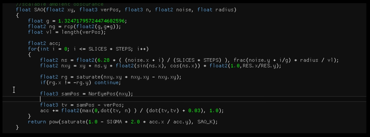 .
.
Hierarhcial Digital Differential Analyzer Global Illumination (HDDAGI)
-
Hierarhcial Digital Differential Analyzer for Efficient Ray-Marching in OpenVDB - 2013 .
-
This is a new global illumination system meant to supersede SDFGI.
-
Key advantages are :
-
Much, much faster. Significantly lower frame time, orders of magnitude faster cascad
-
Generally higher quality (less arctifacting).
-
Much better occclusion (a lot less light leaked).
-
Less memory usage.
It is meant as a drop-in replacement. Should work as a replacement for SDFGI.
-
-
Known issues :
-
For some reason gets DEVICE LOST on Intel GPUs. No idea why.
-
Sharp Reflections not always play good with TAA (wobbly).
-
Darkening (occlusion) on some corners, just like SDFGI. I tried different techniques to see if any worked better. DDGI Octahedral VSM gets rid of them, but also leaks a lot more light, so I am unconvinced. Have other ideas to try, but I don’t have infinite time 🙁
-
SDFGI spherical harmonics turned out to be buggy and not energy conserving. This makes GI look more saturated and have more light than in HDDAGI (which some people may appreciate more), but It’s a bug 😢. Wondering how this can be compensated.
-
Still some further pending optimizations.
-
-
Future :
-
Dynamic object support.
-
High density mode (sub-probes).
-
SDFGI (Signed Distance Field Global Illumination)
-
"SDFGI Solving the accessible Global Illumination problem in Godot" - Outubro 2022 .
-
This paper is absolutely important to understand how SDFGI was made.
-
Requirements
-
Easy to use (no scene or object setup at import time, no setting up SDF, cards,
-
lightmaps, etc). Ideally enable with one click, no set-up.
-
Real-time (or at least fast updates).
-
Good enough quality (no light leaks -or keep to minimum-).
-
Supports both diffuse and reflected light.
-
Supports light into transparent objects.
-
Works as source of light for volumetric fog.
-
Works in all hardware that supports Vulkan, even IGP.
-
Can work in VR (so, using TAA is not required).
-
-
Sacrifices
-
Not the best possible quality (high frequency GI missing, has to be compensated with screen space lighting).
-
Poor dynamic object support (dynamic objects get light from environment, but don't contribute to it). Light blocking may be added to some extent in the future.
-
Needs to use cascades.
-
Limited amount of samples means small emissive objects are spotty.
-
-
Previous work
-
Uses DDGI by Morgan McGuire as a base.
-
Uses Signed Distance Fields generated with Jump Flood .
-
-
-
Signed Distance Fields Dynamic Diffuse Global Illumination - 2020 .
-
Global Illumination (GI) is of utmost importance in the field of photo-realistic rendering. However, its computation has always been very complex, especially diffuse GI. State of the art real-time GI methods have limitations of different nature, such as light leaking, performance issues, special hardware requirements, noise corruption, bounce number limitations, among others. To overcome these limitations, we propose a novel approach of computing dynamic diffuse GI with a signed distance fields approximation of the scene and discretizing the space domain of the irradiance function. With this approach, we are able to estimate real-time diffuse GI for dynamic lighting and geometry, without any precomputations and supporting multi-bounce GI, providing good quality lighting and high performance at the same time. Our algorithm is also able to achieve better scalability, and manage both large open scenes and indoor high-detailed scenes without being corrupted by noise.
-
-
My opinions :
-
Knowing the Godot implementation, I find the visuals simply uninspiring.
-
It sounds bad for me to go for this solution when I didn't even use this for Godot games.
-
I've always found the performance somewhat poor, but it could simply be the low-quality implementation in the editor.
-
-
It’s not screen-space (since it doesn’t rely only on what’s visible on screen).
-
It’s also not a full path-traced solution; instead it’s a form of voxel-based GI accelerated by signed distance fields.
-
Future in Godot :
-
SDFGI will be replaced either way as it has many limitations that can't be resolved (such as slow cascade generation speed).
-
A bounded GI implementation to supersede VoxelGI may be added in the future, but it's not guaranteed.
-
There are plans to replace it with HDDAGI.
-
-
SDFGI vs VoxelGI :
-
SDFGI provides better real-time ability than baked lightmaps, but worse real-time ability than VoxelGI.
-
SDFGI supports dynamic lights, but not dynamic occluders or dynamic emissive surfaces.
-
-
Using Use Occlusion has a small performance cost, but it often results in fewer leaks compared to VoxelGI.
-
Newer on Godot, when compared to VoxelGI. SDFGI was implemented as a new feature in Godot 4.0 release.
-
-
-
SDFGI is something akin to a dynamic real-time lightmap (but it does not requiere unwrapping, nor does it use textures). It’s enabled and it automatically works by generating global illumination for static objects. It does not require raytracing, and it runs in most current (and some years old) dedicated GPUs, even medium-end budget CPUs from some years ago (SDFGI was developed and tested on a GeForce 1060, running at a stable 60 FPS).
-
Light changes are real-time , meaning any change in lighting conditions will result in an immediate update . Dynamic objects are supported only for receiving light from the environment, but they don’t contribute to lighting. Some degree of support is planned for this eventually, but not immediately.
-
SDFGI also supports specular reflections, both sharp and rough , so full PBR scenes should “just work”. In the image below you can see both of them in checkerboard roughness texture.
-
SDFGI is mostly leak free, unlike VCT techniques which are the most common in use today (like SVOGI/GIProbe/etc). As long as walls are thicker than a voxel for a given cascade, light won’t go through.
-
Leaks can be reduced significantly by enabling the Use Occlusion property.
-
-
GI level of detail varies depending on the distance between the camera and surface.
-
Caviats / Issues :
-
Cascade shifts may be visible when the camera moves fast. This can be made less noticeable by adjusting the cascade sizes or using fog.
-
Good reflections and indirect lighting, but beware of leaks and visible cascade shifts.
-
SDFGI has some downsides due to its cascaded nature. When the camera moves, cascade shifts may be visible in indirect lighting.
-
This can be alleviated by adjusting the cascade size, but also by adding fog (which will make distant cascade shifts less noticeable).
-
-
Performance will suffer if the camera moves too fast. This can be fixed in two ways:
-
Ensuring the camera doesn't move too fast in any given situation.
-
Temporarily disabling SDFGI in the Environment resource if the camera needs to be moved at a high speed, then enabling SDFGI once the camera speed slows down.
-
-
When SDFGI is enabled, it will also take some time for global illumination to be fully converged (25 frames by default). This can create a noticeable transition effect while GI is still converging.
-
To hide this, you can use a ColorRect node that spans the whole viewport and fade it out when switching scenes using an AnimationPlayer node.
-
-
The signed distance field is only updated when the camera moves in and out of a cascade. This means that if geometry is modified in the distance, the global illumination appearance will be correct once the camera gets closer. However, if a nearby object with a bake mode set to Static or Dynamic is moved (such as a door), the global illumination will appear incorrect until the camera moves away from the object.
-
SDFGI's sharp reflections are only visible on opaque materials. Transparent materials will only use rough reflections, even if the material's roughness is lower than 0.2.
-
-
Performance :
-
The number of cascades can be adjusted to balance performance and quality. The number of rays thrown per frame can be adjusted in the Project Settings. The rendering can optionally be performed at half resolution (and then linearly scaled) to improve performance significantly.
-
-
Setting up :
-
Make sure your MeshInstance nodes have their Global Illumination > Mode property set to Static in the inspector.
-
Any Mesh can receive Indirect Lighting, but only static meshes can contribute to Indirect Lighting.
-
For meshes:
-
Disabled:
-
The mesh won't be taken into account in SDFGI generation. The mesh will receive indirect lighting from the scene, but it will not contribute indirect lighting to the scene.
-
-
Static (default):
-
The mesh will be taken into account in SDFGI generation. The mesh will both receive and contribute indirect lighting to the scene. If the mesh is changed in any way after SDFGI is generated, the camera must move away from the object then move back close to it for SDFGI to regenerate. Alternatively, SDFGI can be toggled off and back on. If neither is done, indirect lighting will look incorrect.
-
-
Dynamic (not supported with SDFGI):
-
The mesh won't be taken into account in SDFGI generation. The mesh will receive indirect lighting from the scene, but it will not contribute indirect lighting to the scene.
-
This acts identical to the Disabled bake mode when using SDFGI.
-
-
-
For lights:
-
Disabled:
-
The light will not be taken into account for SDFGI baking. The light won't contribute indirect lighting to the scene.
-
-
Static:
-
The light will be taken into account for SDFGI baking. The light will contribute indirect lighting to the scene. If the light is changed in any way after baking, indirect lighting will look incorrect until the camera moves away from the light and back (which causes SDFGI to be baked again). will look incorrect. If in doubt, use this mode for level lighting.
-
-
Dynamic (default):
-
The light won't be taken into account for SDFGI baking, but it will still contribute indirect lighting to the scene in real-time. This option is slower compared to Static . Only use the Dynamic global illumination mode on lights that will change significantly during gameplay.
-
-
-
-
Add a WorldEnvironment node and create an Environment resource for it.
-
Edit the Environment resource, scroll down to the SDFGI section and unfold it.
-
Enable SDFGI > Enabled .
-
SDFGI will automatically follow the camera when it moves, so you do not need to configure extents (unlike VoxelGI).
-
-
To make a specific light emit more or less indirect energy without affecting the amount of direct light emitted by the light, adjust the Indirect Energy property in the Light3D inspector.
-
It is not a screen-space effect, so it can provide global illumination for off-screen elements (unlike SSIL).
-
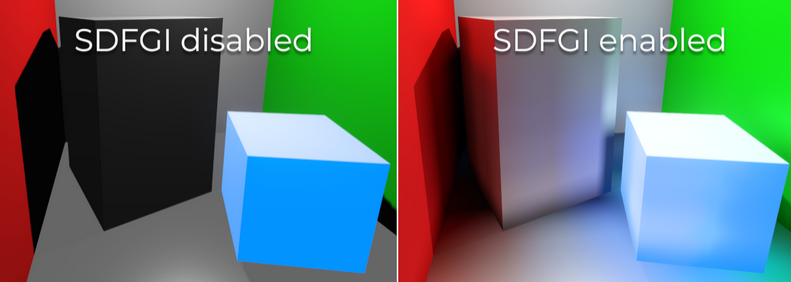 .
.
-
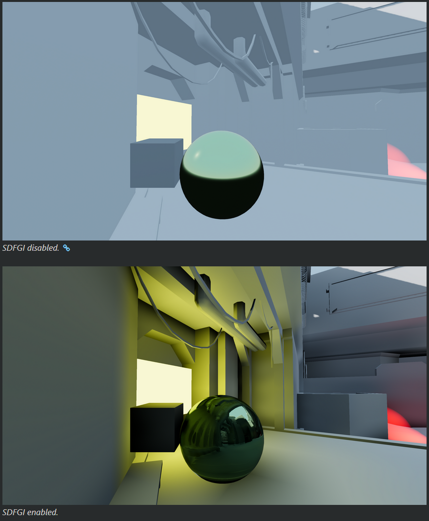 .
.
Lighting Grid Hierarchy
-
Lighting Grid Hierarchy for Self-illuminating Explosions - Siggraph 2017 .
-
Focusing on temporal coherency to avoid flickering in animations, we introduce lighting grid hierarchy for approximating the volumetric illumination at different resolutions. Using this structure we can efficiently approximate the lighting at any point inside or outside of the explosion volume as a mixture of lighting contributions from all levels of the hierarchy. As a result, we are able to capture high-frequency details of local illumination, as well as the potentially strong impact of distant illumination. Most importantly, this hierarchical structure allows us to efficiently precompute volumetric shadows, which substantially accelerates the lighting computation. Finally, we provide a scalable approach for computing the multiple scattering of light within the smoke volume using our lighting grid hierarchy.
-
Ray tracing can be layered on top for visibility injection, but the technique itself does not depend on it.
-
Lighting Grid Hierarchy with Raytracing Hardware Demo .
-
100k VPL (100.000 Virtual Point Lights).
-
Screen-Space Directional Occlusion (SSDO)
Precomputed Radiance Transfer (PRT)
-
My understanding :
-
Based on the explanations in "A Data-Driven Paradigm for Precomputed Radiance Transfer - 2022" and "Neural Precomputed Radiance Transfer - 2022", I understood that this strategy is an intermediate between baking and dynamic.
-
The idea would be to compute different types of lighting on a mesh, choosing which to apply based on the mesh's current direct lighting conditions.
-
It uses Spherical Harmonics directly, but another basis can be used.
-
ChatGPT:
-
PRT is a technique that moves expensive, direction-dependent light transport calculations offline so that, at runtime, shading under complex (often dynamic) lighting can be evaluated with a small number of dot-products.
-
-
-
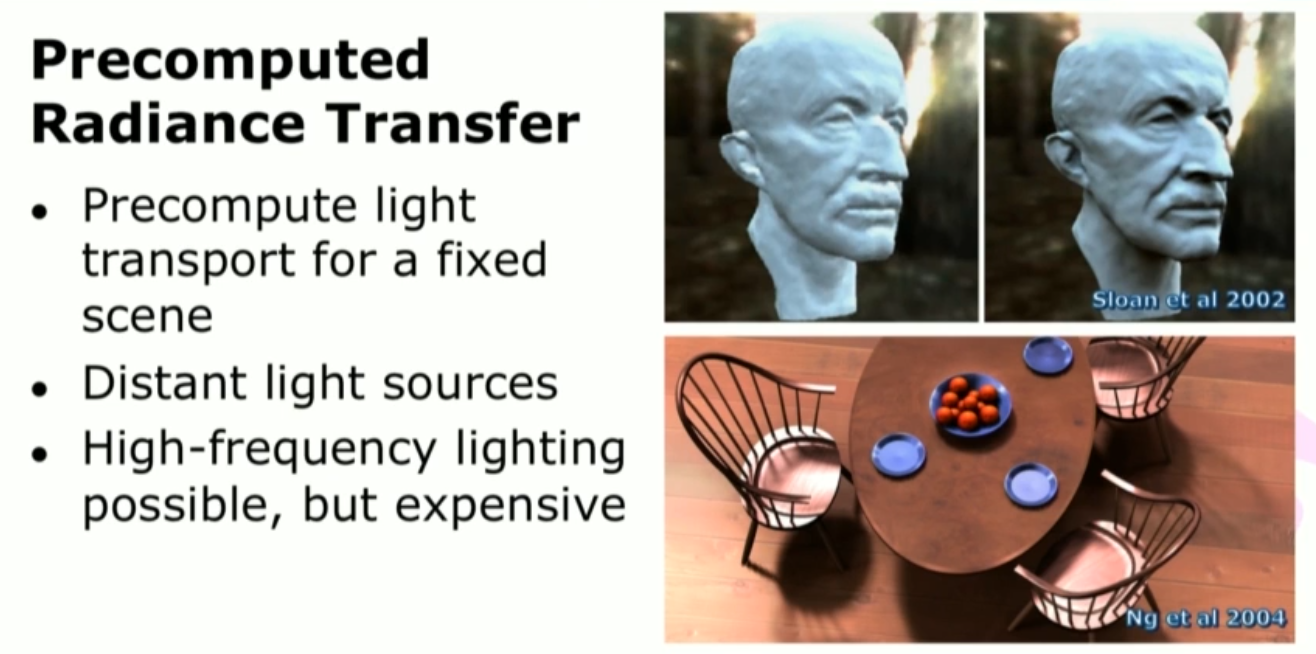 .
.
-
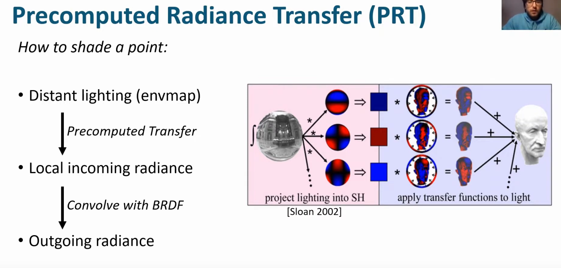 .
.
-
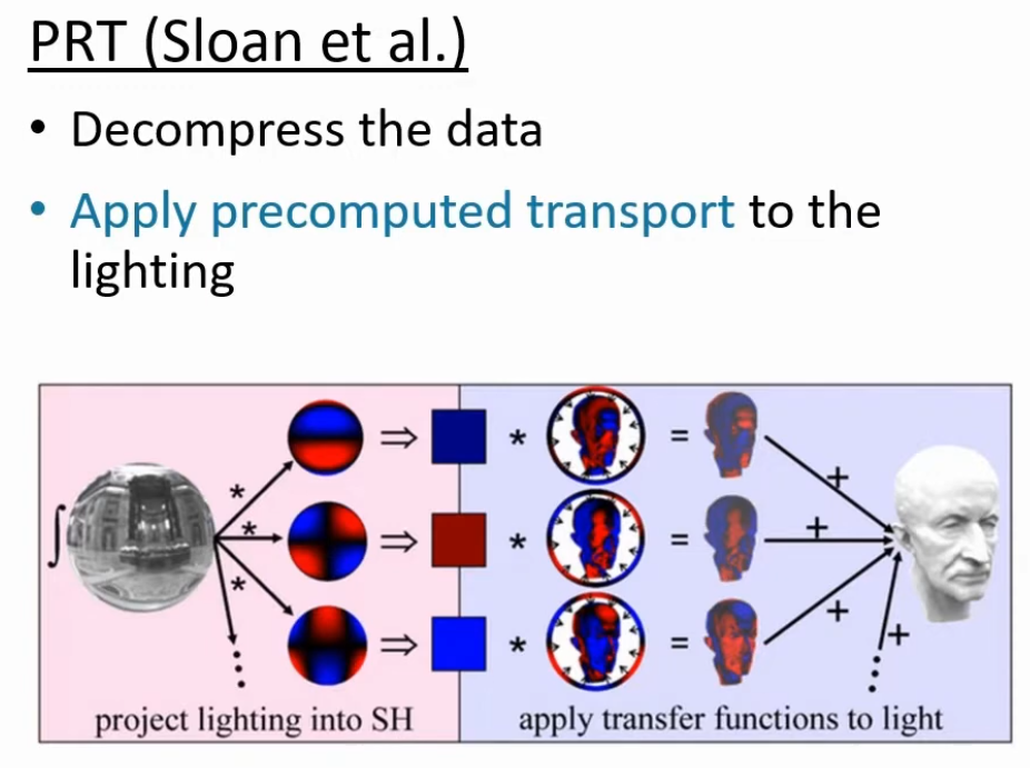 .
.
-
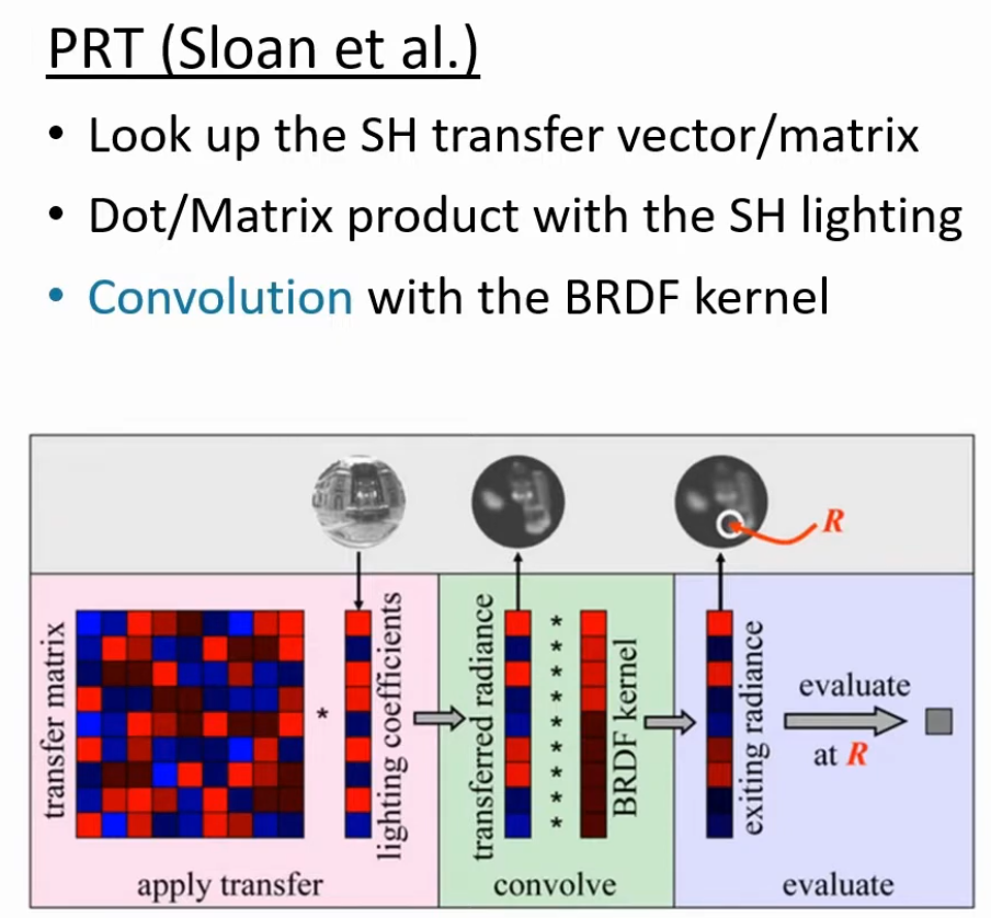 .
.
-
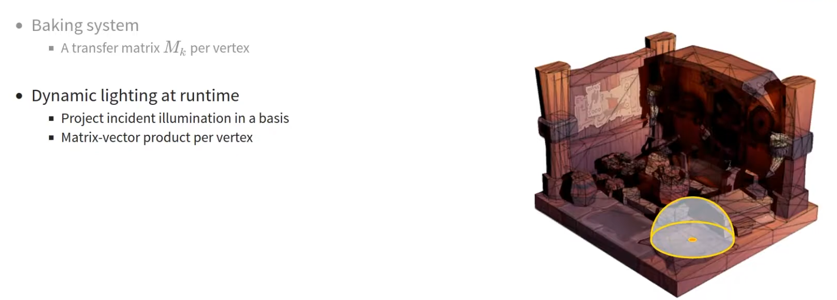 .
.
-
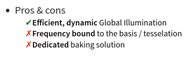 .
.
-
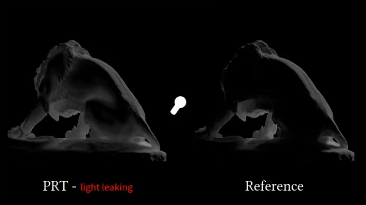 .
.
-
A Data-Driven Paradigm for Precomputed Radiance Transfer - Unity 2022 .
-
A Data-Driven Paradigm for Precomputed Radiance Transfer - Unity 2022 .
-
Very interesting.
-
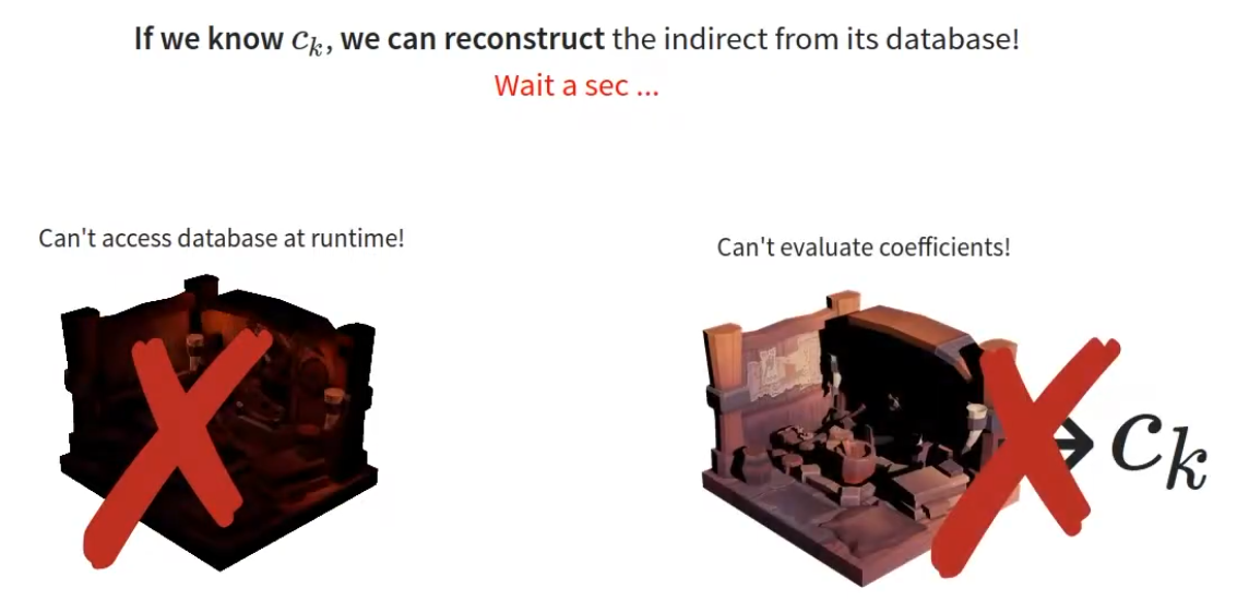 .
.
-
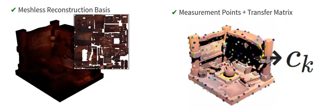 .
.
-
-
Neural Precomputed Radiance Transfer - 2022 .
-
Neural PRT:
-
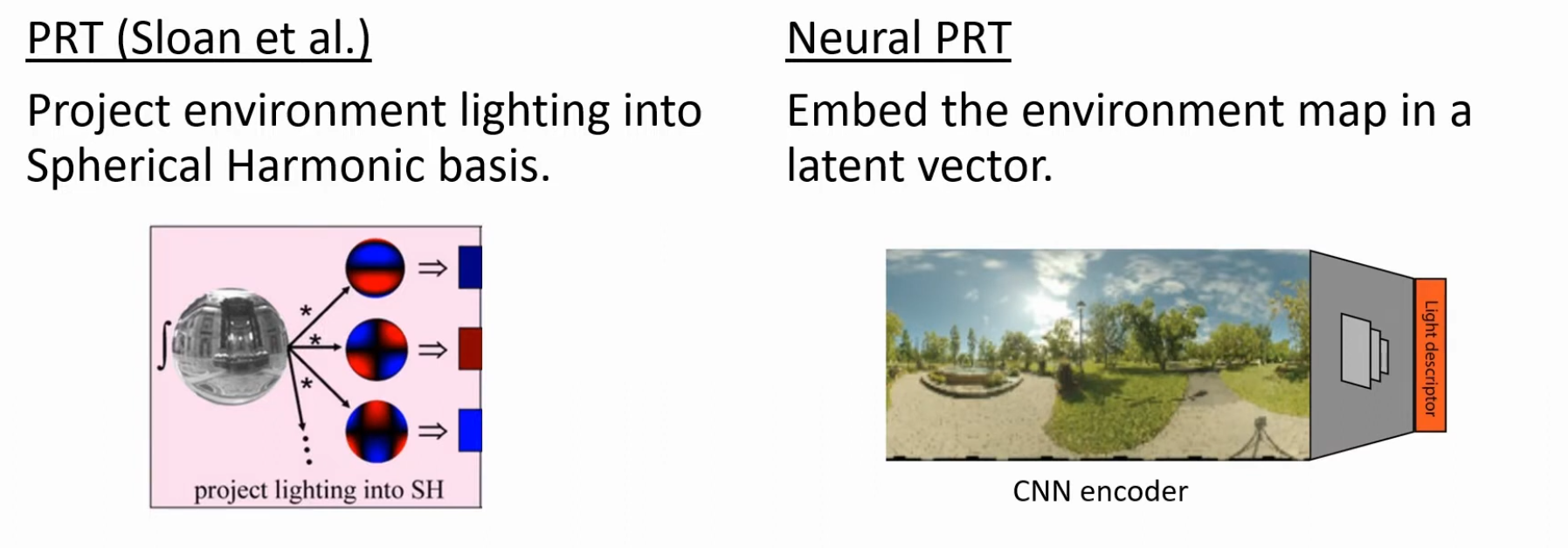 .
.
-
A CNN encoder is the part of a convolutional neural network (CNN) that compresses input data into a compact, meaningful representation called a latent representation. It functions by progressively down-sampling and extracting hierarchical features from the input, such as an image, through a series of convolutional and pooling layers. The goal of the encoder is to reduce the input's dimensionality while retaining essential information, making it a compressed version of the original data that can then be used by a decoder for tasks like reconstruction or pixel-level prediction
-
-
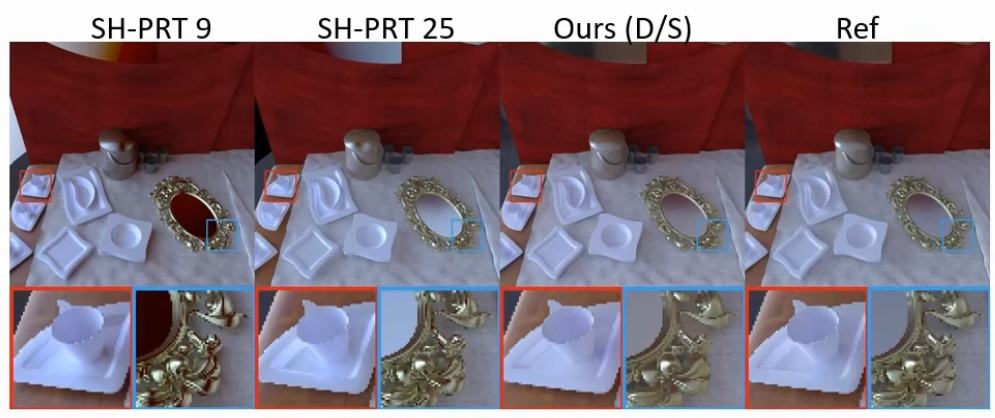 .
.
-
"Even with 5 circle harmonic bands (25 coefficients), spherical harmonics tend to cutoff the high frequency angular signals, this is visible on the mirror, for example".
-
-
-
Instead of dealing with rays, PRT deals with functions on a sphere.
-
Traditional PRT suggests as choice of basis:
-
Spherical Harmonics
-
Haar Wavelets.
-
Spherical Gaussians.
-
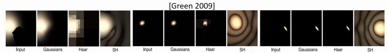 .
.
-
-
The choice of basis has been one of the main domains of research.
-
Usage :
-
It is designed for static geometry (or limited deformation) and is primarily targeted at low-frequency environment lighting and shadowing / soft interreflection effects that can be precomputed.
-
Partially replaced by real-time ray-tracing / dynamic probe systems for workflows that require runtime changes. PRT is efficient for low-frequency, mostly-static content (precomputation), but for highly dynamic environments engines increasingly use real-time methods (RT + denoising, probe volumes) to handle scene changes.
-
-
PRT Probes - The Division 1 - 2016 .
-
It is not normal PRT, but rather PRT Probes.
-
I watched about the first 20 minutes and some other segments of the video.
-
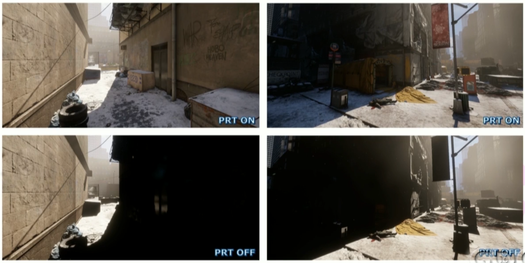 .
.
-
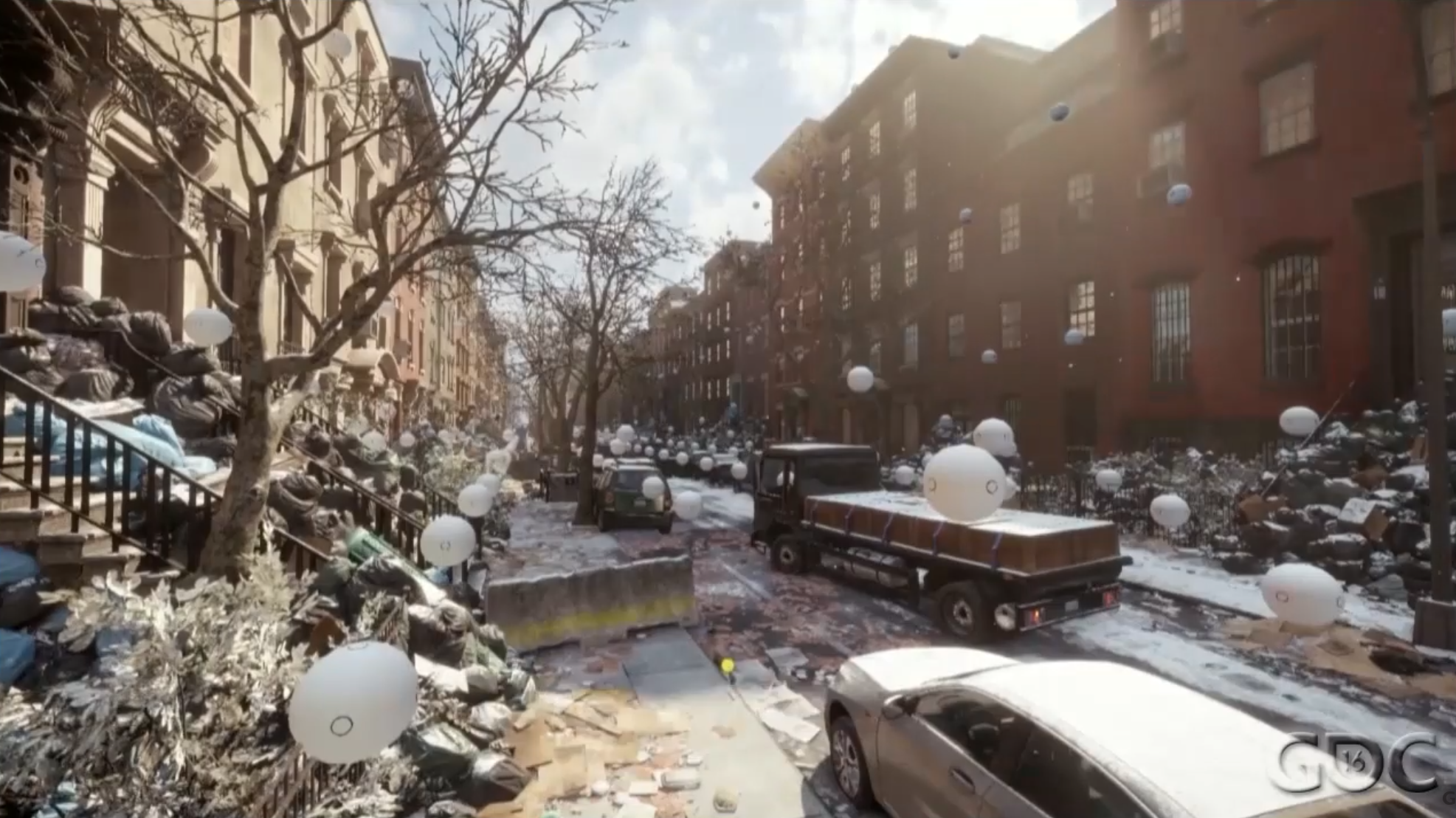
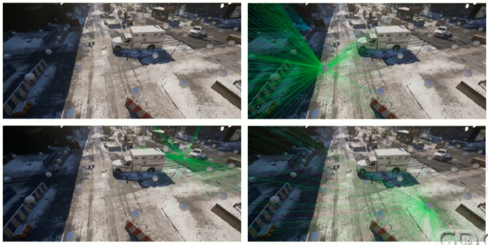 .
.
-
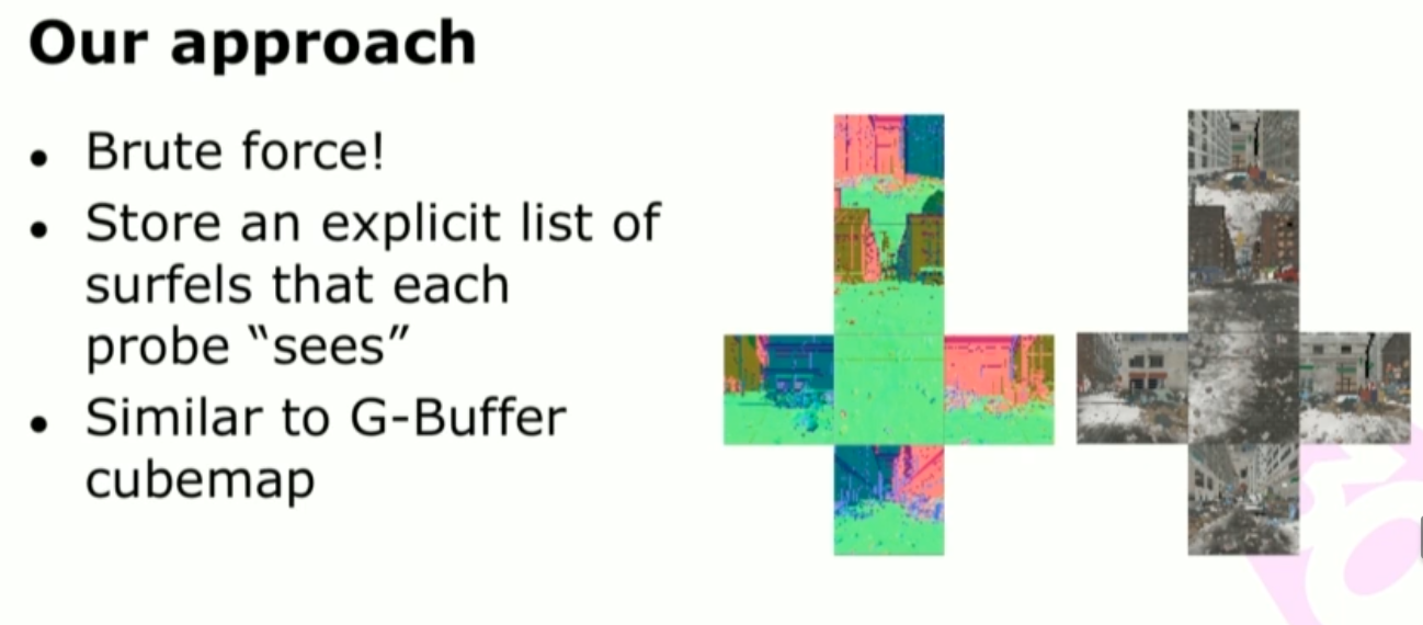 .
.
-
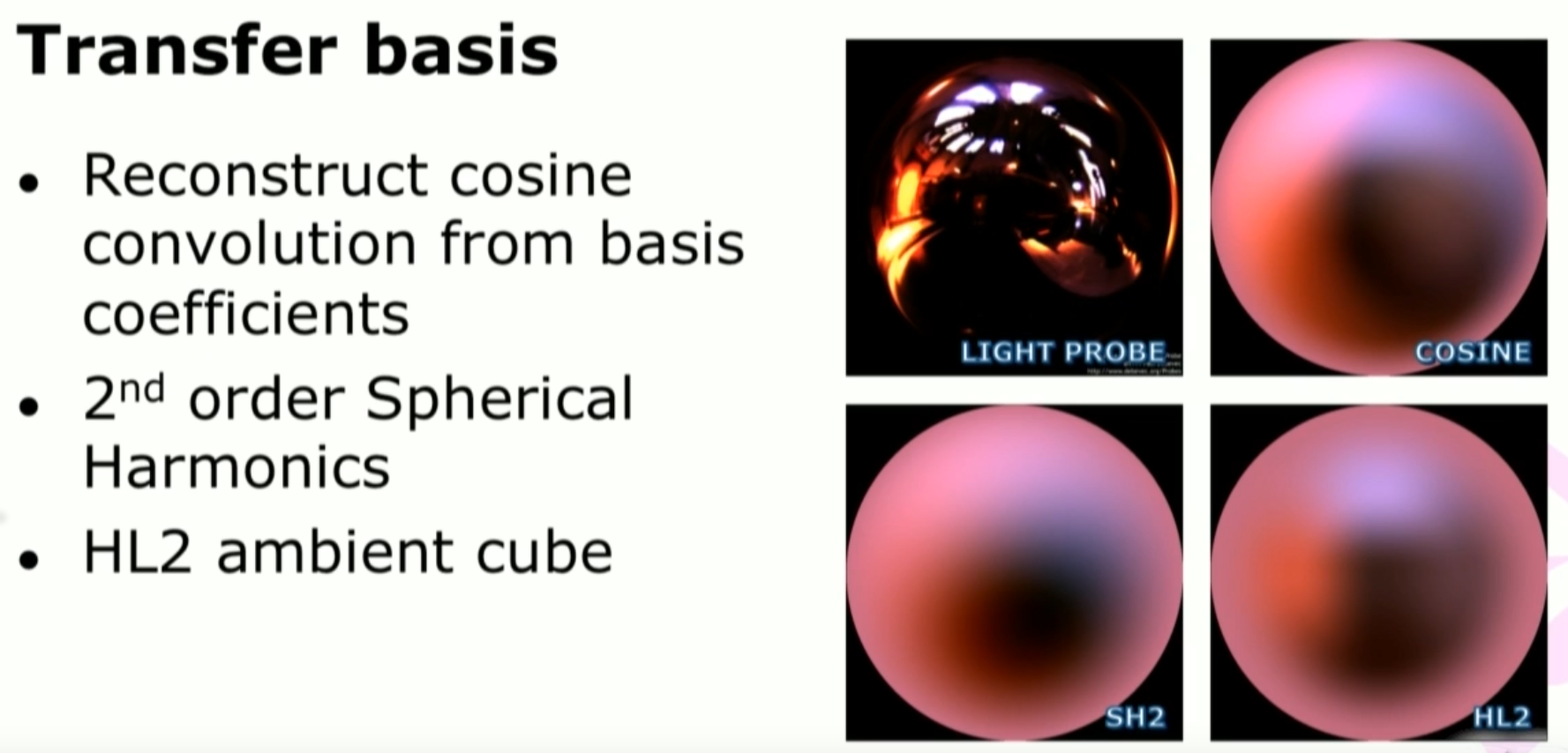 .
.
-
After considerations, we settled on the Half Life 2 Ambient Cube Basis (HL2), which is not a real basis but 6 vectores aligned; so it requires only six floats.
-
-
The probes are placed automatically via a 4x4 meters raycast grid, spawning a probe on every ray hit; also, spawn probes alongside building walls, to avoid them looking flat.
-
The storage on disk is via a 2D grid with 64x64 meters, with maximum of 1000 probes, but usually 200 probes per sector. The sectors are streamed in and out as the player moves.
-
 .
.
-
 .
.
-
Manhattan == Manhattan city map.
-
-
Voxel Ambient Occlusion (VXAO)
-
Not in screen space.
-
Unlike VXGI which controls all illumination, VXAO is only utilized for Ambient Occlusion, enabling us to integrate it into a wider array of games and game engines that use traditional illumination technologies.
-
It’s more accurate than SSAO and its derivatives, casts deeper, richer shadows that account for even the smallest details in a scene, and runs faster than other competing effects when they’re rendered at a similar quality.
-
Even still, HBAO+’s Ambient Occlusion shadowing is far from the level of fidelity offered by VXAO, which avoids the caveats of screen space techniques, enabling us to deliver the most accurate and realistic Ambient Occlusion shadowing seen to date.
-
With VXAO, occlusion and lighting information is gathered from a ‘world space’ voxel representation of the scene, which takes into account a large area around the viewer. Included in this voxelization are objects and details currently invisible to the viewer, and those behind the viewer, too. The result is scene-wide Ambient Occlusion shadowing, instead of ‘screen space’ shadowing based on what you can currently see. This allows AO shadows to be cast into a scene from objects near to the player but just outside of their view, and from occluded objects in the distance large enough to affect the appearance of the scene.
-
Use on:
-
Rise of the Tomb Raider.
-
MSSAO (Multi-Resolution Screen-Space Ambient Occlusion)
-
 .
.
-
You can combine results from different occlusion radius.
-
It is a technique from a 2010 paper.
SSAO (Screen-Space Ambient Occlusion)
-
“Where should I remove light because it’s blocked?”
-
Ray Traced Ambient Occlusion itself is an approximation of Indirect Light, and SSAO is an approximation of Ray Traced Ambient Occlusion.
-
So it's an approximation of an approximation.
-
-
SSAO only acts on ambient light . It does not affect direct light.
-
Think of SSAO as a shadow-only pass, faking soft contact shadows.
-
Ray Traced AO would be the "correct" ambient occlusion, but that is kinda difficult to say as Ambient Occlusion itself is a "fake term"; SSAO approximates it.
-
It's much faster then Ray Traced AO.
-
Approximates ambient occlusion as a cheap GI term; bent normals can guide diffuse light injection.
-
Screen-space sampling; rasterization-based.
-
-
If you want to force SSAO to work with direct light too, use the Light Affect parameter. Even though this is not physically correct, some artists like how it looks.
-
SSAO looks best when combined with a real source of indirect light, like VoxelGI .
-
-
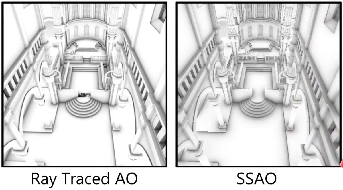 .
.
Combined Adaptive Compute Ambient Occlusion (CACAO)
-
AMD FidelityFX Combined Adaptive Compute Ambient Occlusion .
-
Released in May 2020.
-
As of 2023, it became part of the AMD FidelityFX SDK.
-
Updated in May 2025.
-
"Artist control, etc, but deviates from the rendering equation".
Screen-Space Global Illumination Based-Invariance (SSVGI)
-
The author of Radiance Cascading worked on this technique for PoE1.
-
Uses exclusively image space data.
-
Calculates GI for every point from scratch.
-
Still needs denoising.
-
Uses Screen Space Shadow Hierarchy.
-
"Shadow cascade".
-
Light Propagation Volumes (LPV)
-
First introduced by Crytek in 2009.
-
LV calculation of global illumination consists of three steps:
-
Injection virtual points lights obtained from Reflective Shadow Maps into LPV 3D grid.
-
Propagation of light intensity in grid stored in spherical harmonics coefficients.
-
Lookup for light intensity in LPV while scene rendering.
-
-
LPV sits in the same family as Voxel-GI (both use a 3D grid) and is functionally closer to runtime probe/volume methods like DDGI than to precomputed PRT — but LPV’s propagation approach and data layout make its behavior and trade-offs distinct.
-
Inject light into a 3D regular grid (the “volume”) from direct light sources or from virtual point lights / reflective shadow maps. The injected values are usually stored as low-order spherical harmonics (SH) or simple directional bands per cell.
-
Iteratively propagate those values between neighboring grid cells (a diffusion / scattering sweep). The propagation step moves energy through the grid and approximates multiple diffuse bounces.
-
At shading time, the renderer samples the grid (trilinear / tetrahedral interpolation) and uses the sampled radiance/SH to illuminate surfaces (usually only the diffuse term).
-
-
Key implementation notes: LPV normally stores very low angular detail (few SH bands or directional channels) and relies on repeated propagation iterations to spread light. It does not explicitly store full scene geometry inside the grid (although depth/normal heuristics can be used to reduce obvious leakage).
-
Usage :
-
LPV fell out of favor in many production engines because its core design produces persistent, hard-to-fix artifacts (notably light bleeding and poor directional fidelity) and because alternative runtime GI approaches (probe-based DDGI variants, voxel-cone tracing, and hardware-accelerated ray-traced GI) offer better trade-offs for modern, dynamic scenes and artist workflows. The choice is engineering- and platform-dependent; LPV still makes sense in limited cases (very low-cost, low-frequency indirect lighting), but it is no longer the common “go-to” for high-quality dynamic GI in AAA engines.
-
-
-
Deprecated in UE5, used in UE4.
-
Ambient Color
-
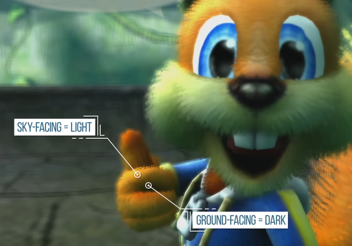 .
.
-
Usually 2 colors, applied depending on the normal of the surface.
Instant Radiosity ("Virtual Lights")
-
It's not instant, and has nothing to do with the 'Radiosity' method.
-
-
Approximates GI by spawning virtual point lights (VPLs) from primary light bounces.
-
Then renders the scene lit by these many point lights (with importance sampling and clamping to reduce artifacts).
-
It’s an approximation to many-bounce light transport.
-
The method requires finding secondary bounces to spawn virtual point lights (VPLs). This is traditionally done with ray tracing.
-
However, simplified rasterization approximations (e.g., reflective shadow maps) exist that avoid explicit ray casting.
-
-
A "Light Source" is the Sun, and a "Virtual Light" is the Moon.
-
Starting from the light source, generate virtual lights placed where the light illuminates a surface, by sampling random directions from the light source.
-
The virtual lights account for indirect illumination; the indirect illumination becomes direct illumination from the virtual lights.
-
It converts the problem of indirect illumination into the problem of rendering many light sources.
-
It can account for one or many bounces of light; you just need to keep creating virtual lights.
-
This is the opposite of Path Tracing; it's called Light Tracing .
-
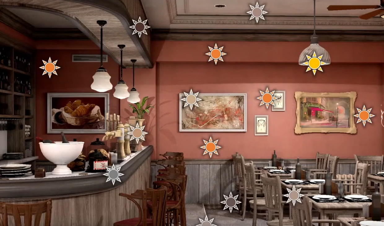 .
.
-
CryEngine 3:
-
This class of approaches is based on the idea of representing indirect lighting as a cloud set of virtual point light sources (VPL). Consequently, this technique has a great potential to speed up with GPU. Its main advantages are good veracity and absence of any scene/lighting/camera constraints. Unfortunately, the main disadvantage of these methods is inadequate performance primarily because of the necessity to render at least 300-400 shadow- casting VPLs for an arbitrary scene to represent the precise solution without artifacts and flickering.
-
Horizon-Based Ambient Occlusion (HBAO)
-
"Image-Space Horizon-based Ambient Occlusion" - Nvidia Siggraph 2008.
-
Very expensive trigonometry operations and too slow at the time.
Alchemy Screen-Space Ambient Obscurance (AlchemyAO)
-
HBAO+ is an optimization of this technique.
Metropolis Light Transport (MLT)
-
Siggraph 1997.
-
Monte Carlo method that explores light paths in a “mutation” process, emphasizing important contributions (e.g., caustics).
-
Ray tracing-based Monte Carlo.
Path Tracing
-
Ray Tracing, Path Tracing, Global Illumination, BVH .
-
Great video. Very illustrative.
-
Path Tracing and Global Illumination:
-
Nothing "new" in the explanations. It's based on a lot of material I studied.
-
Sometimes it complicates some explanations, making things seem a bit magical and "untouchable"
-
-
BVH: Binary Volume Hierarchy.
-
Maybe it's the most relevant explanation.
-
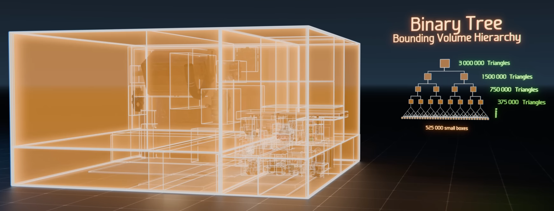 .
.
-
-
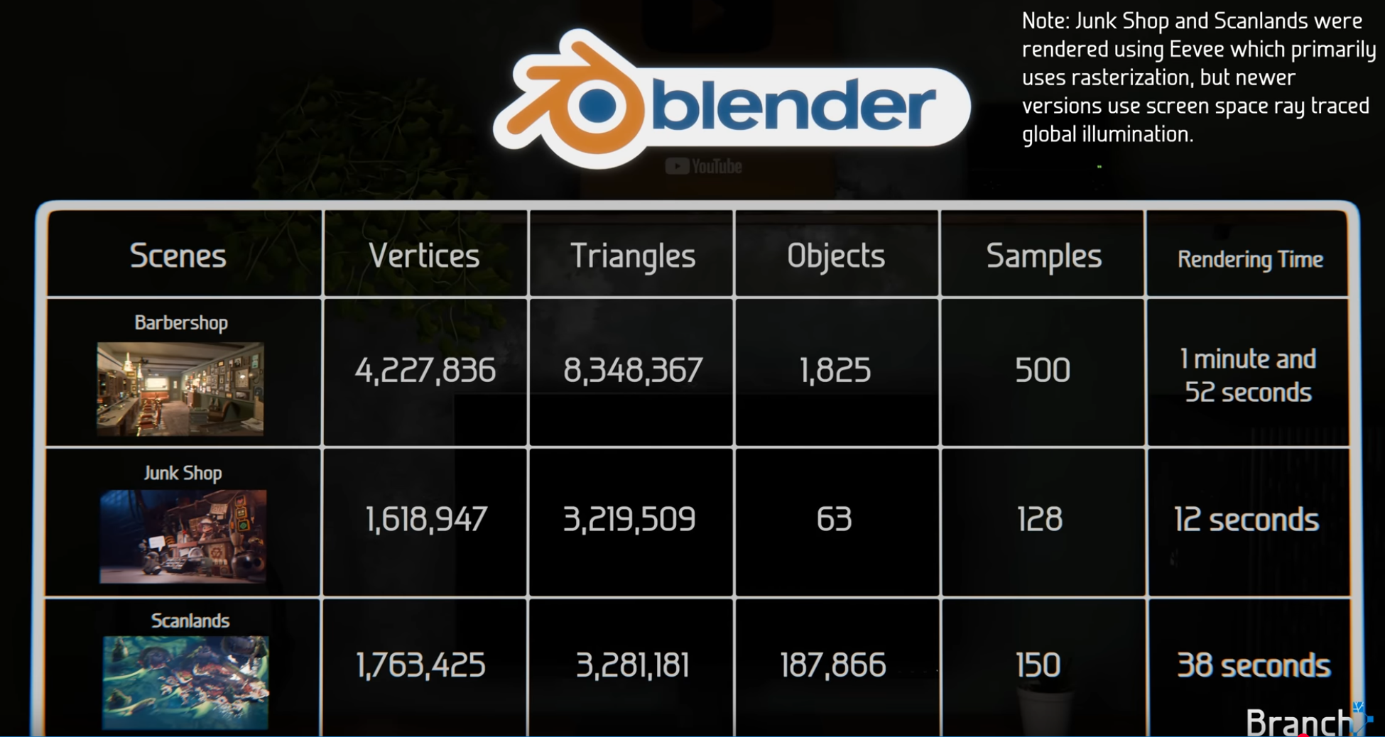 .
.
-
Interesting performance statistics.
-
-
The video ends at 22:15.
-
-
The standard method for computing global illumination today.
-
Finds light paths starting from the camera .
-
Project a ray and pick a random direction.
-
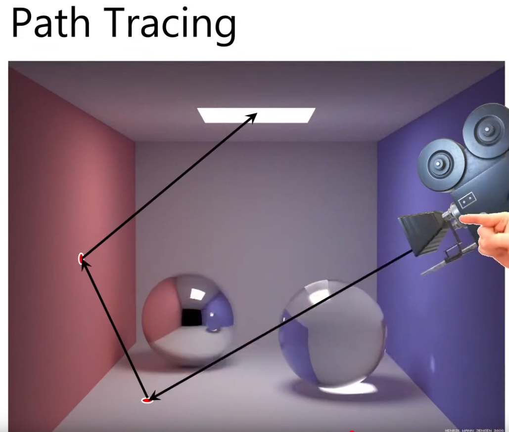
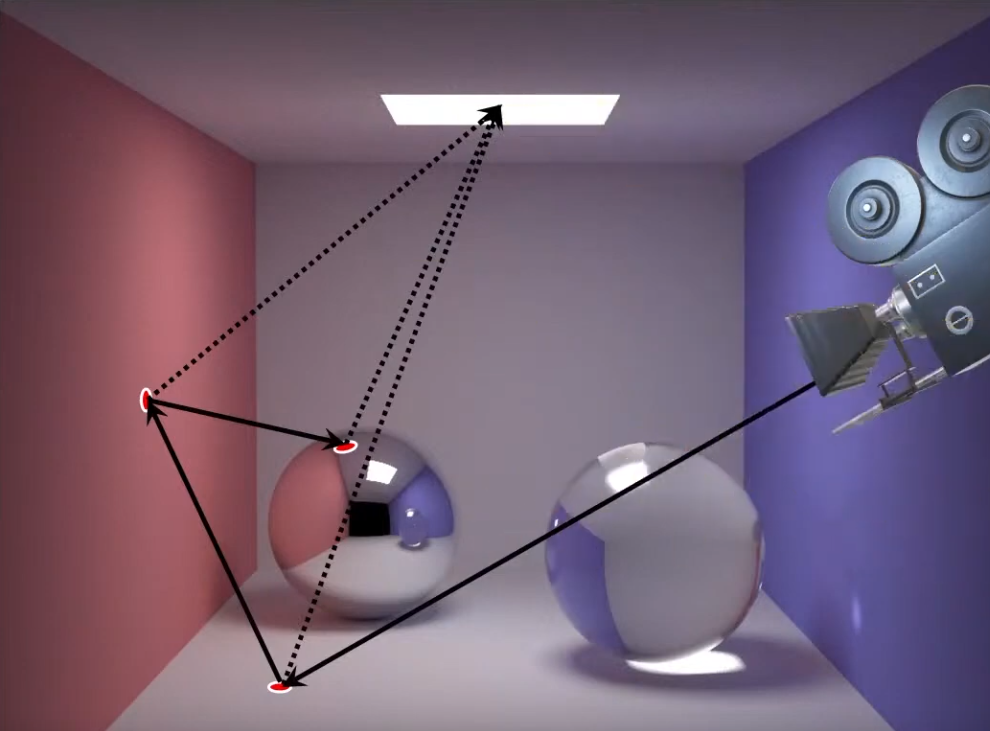 .
.
-
It tries to find all possible light paths starting from the camera to the light source.
-
The amount of light paths consider is indicated by the SPP (Samples Per pixel).
-
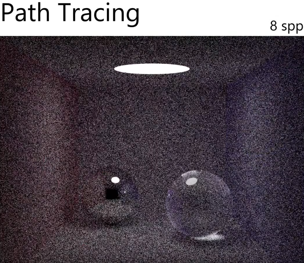
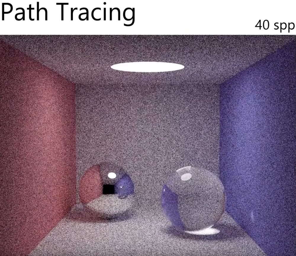
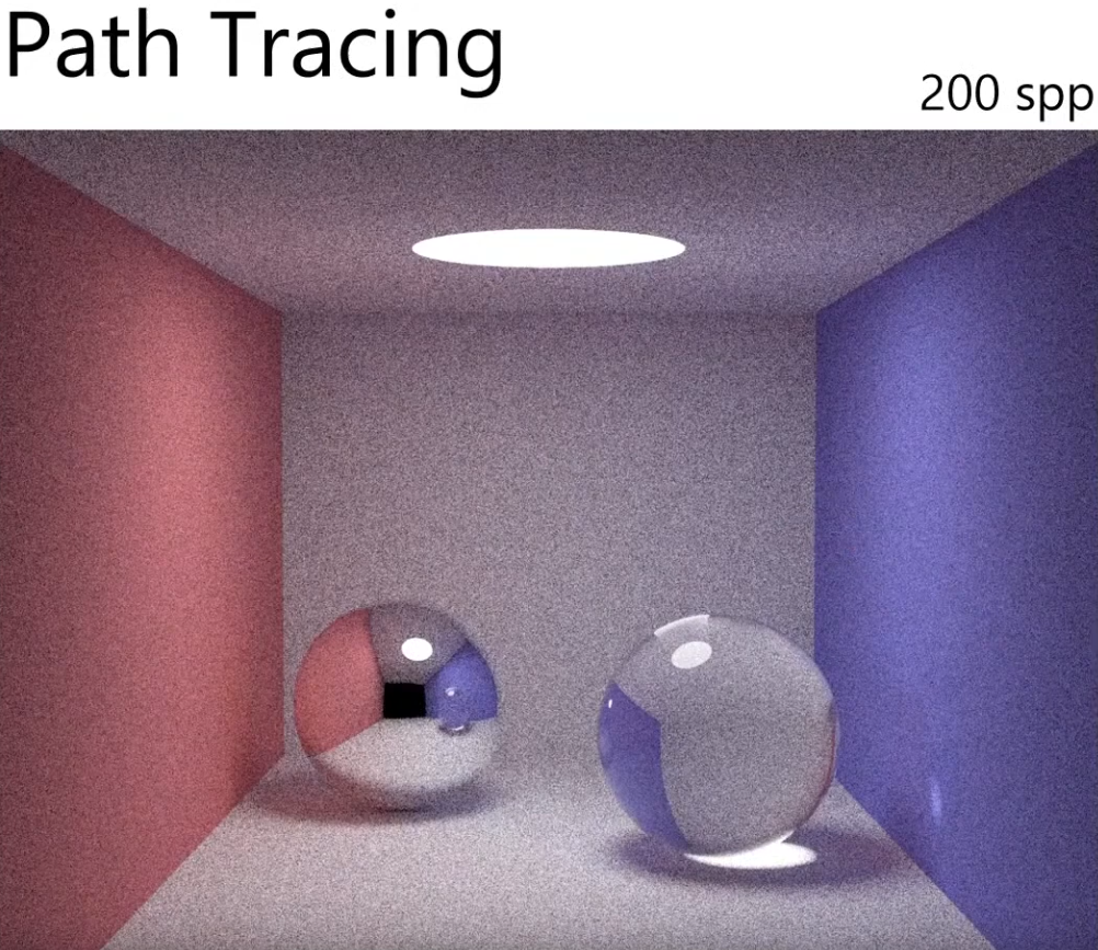
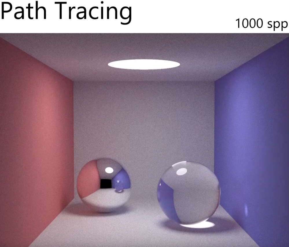
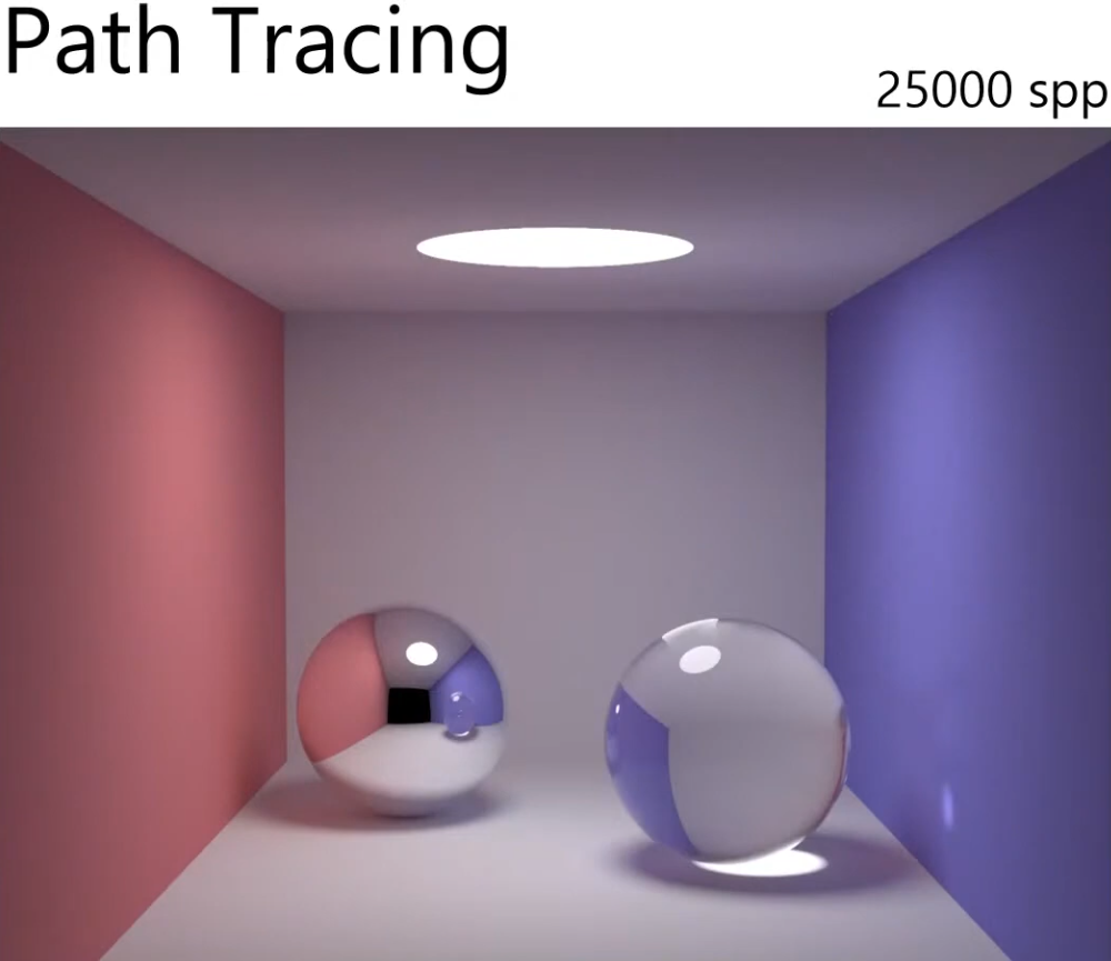 .
.
-
Denoiser :
-
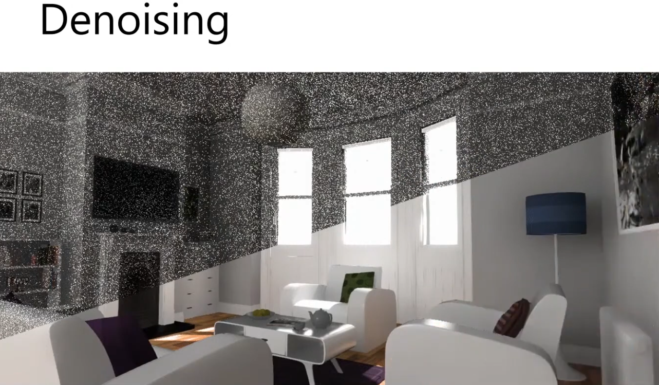 .
.
-
-
Use the samples from the neighboring pixels, to estimate the indirect illumination for the current pixel.
-
AI and Deep Learning is used today.
-
Spacial Denoising :
-
Temporal Denoising :
-
Cheaper and it doesn't blur.
-
For a game that has a camera moving all the time, you'll have to use:
-
Motion Vectors.
-
How things moved between frames.
-
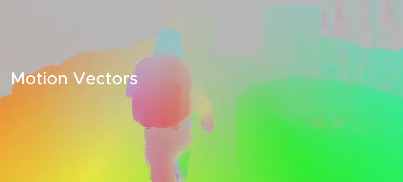 .
.
-
-
Reject samples that were reprojected incorrectly.
-
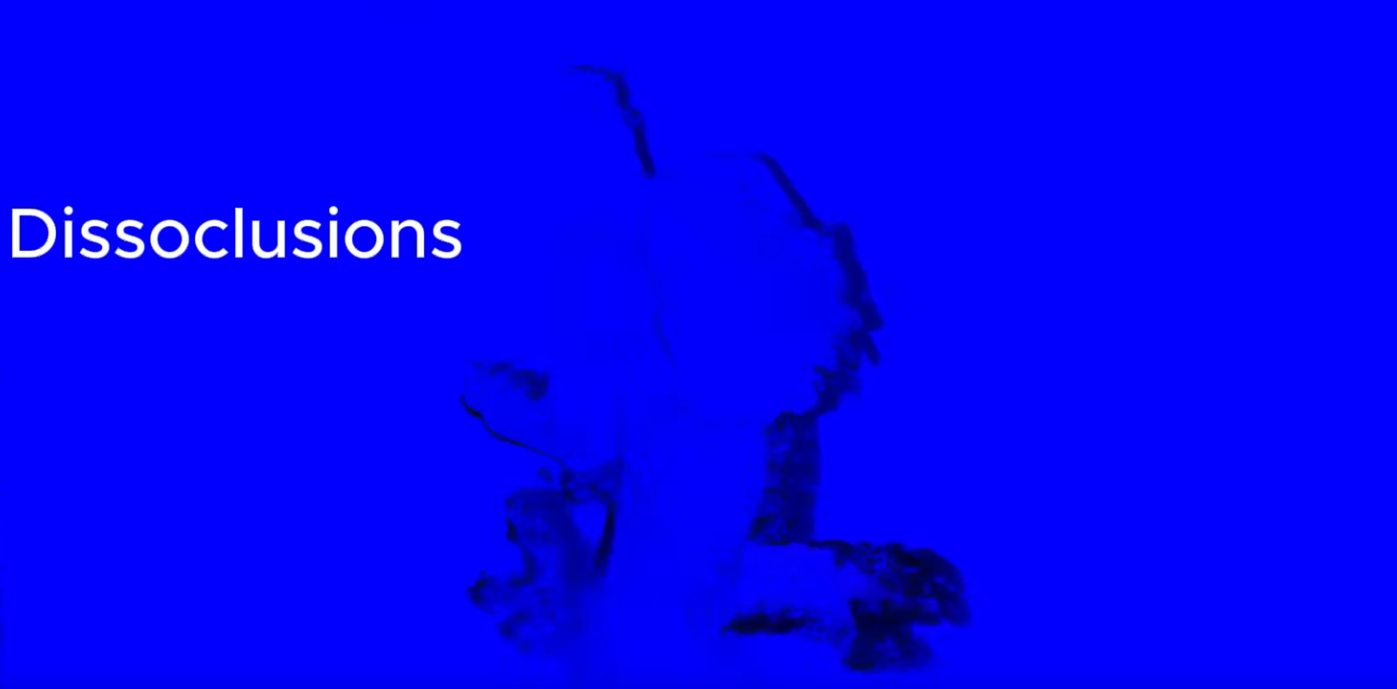 .
.
-
-
-
Joint Bileteral Filter :
-
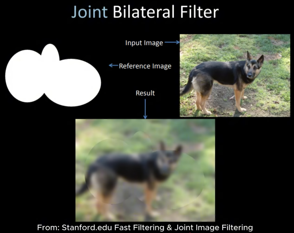 .
.
-
Takes into account the depth and normals.
-
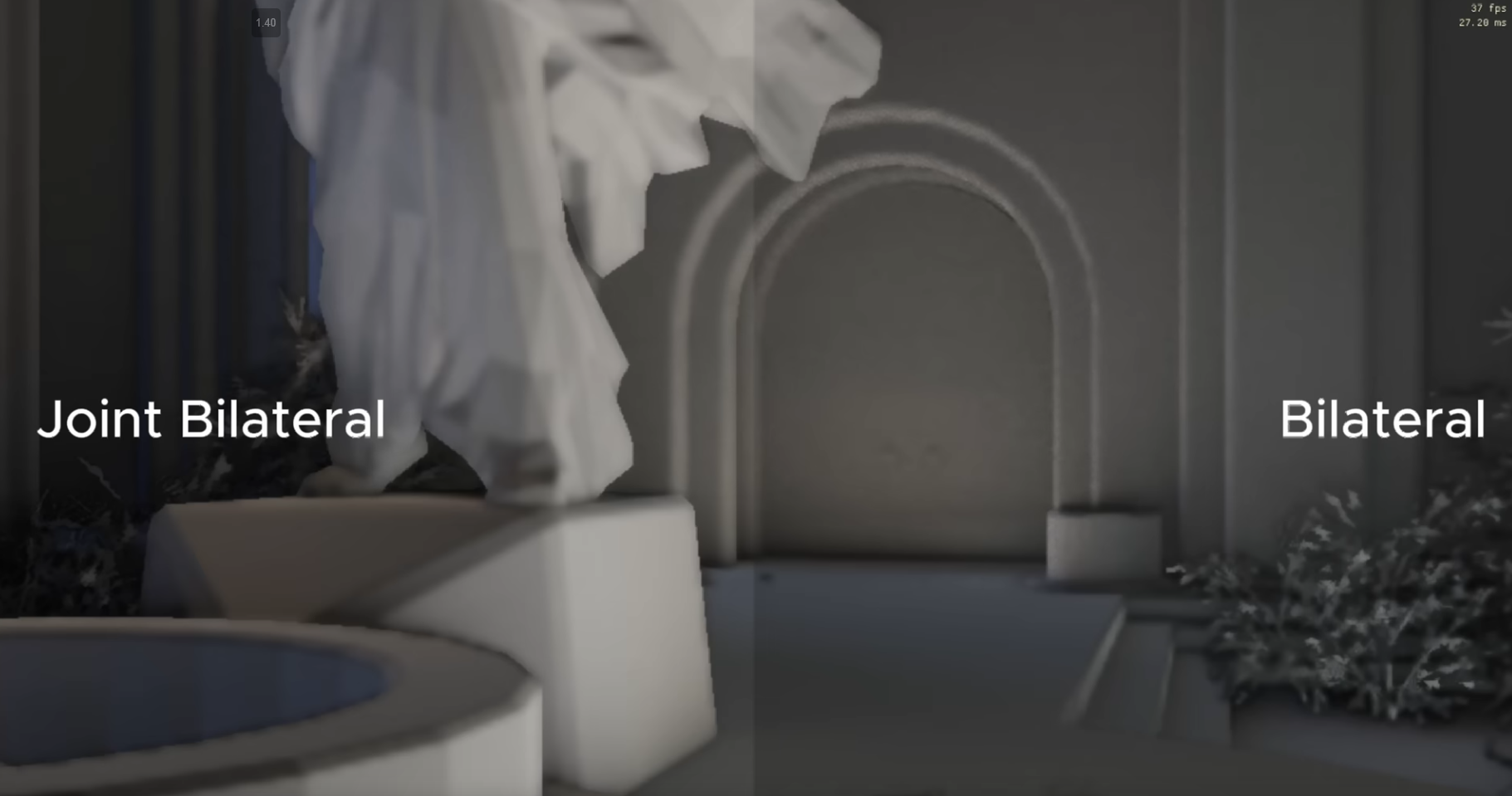 .
.
-
My understanding is that there is less blur based on the depth buffer, in the image on the left.
-
-
-
Photon Mapping
-
1995 to 2001.
-
Two-pass algorithm: first, photons are traced from light sources and stored; second, the radiance is gathered at surfaces to compute illumination.
-
Handles caustics and diffuse interreflections.
-
Uses Ray tracing (photon tracing) + data structure (k-d tree for photon storage).
-
CryEngine 3:
-
These methods are less popular than the others in real-time graphics because of their performance issues. Usually this class of techniques is based on the classical photon-mapping approach. These methods usually use GPU texture fetching and rendering units to accelerate the photon map evaluation. The usual optimizations for these techniques are irradiance caching, importance sampling, and the incremental approach. One drawback of these methods is that the scene needs to be preprocessed to get the unique representation for the photon map. Another problem is photon map updates caused by scene and lighting changes, which leads to highly inconsistent performance and intermittent stalls.
-
Radiosity
-
-
Origin of the Cornell Box .
-
Radiosity is a global illumination method that solves light transport between diffuse-only surfaces by discretizing geometry into patches and solving a linear system of energy exchange.
-
Produces smooth, view-independent GI (often offline or precomputed).
-
Surface-based; patch-to-patch energy exchange (matrix solve). Ray tracing is optional for visibility (hemicube or ray casting).
-
It doesn't use ray tracing inherently. Radiosity is based on solving a radiosity matrix (energy exchange between surface patches).
-
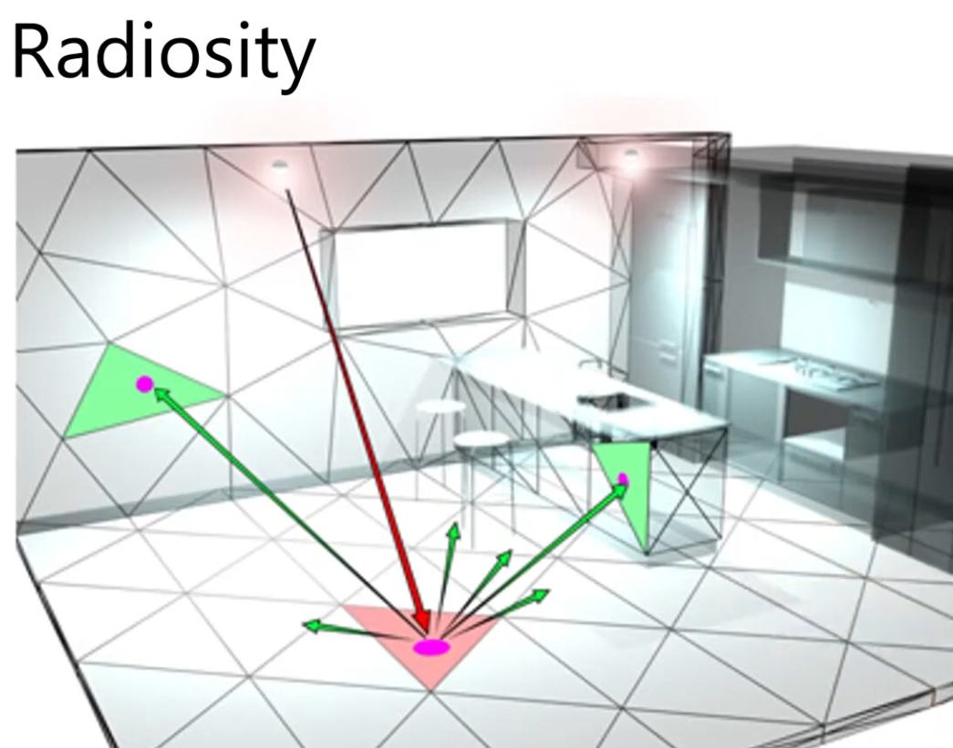 .
.
-
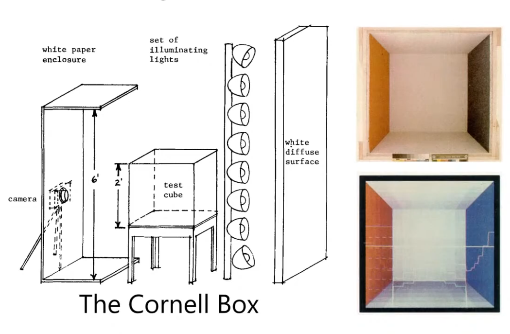 .
.
-
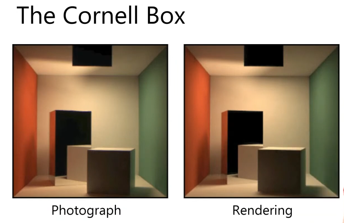 .
.
Lightmaps
-
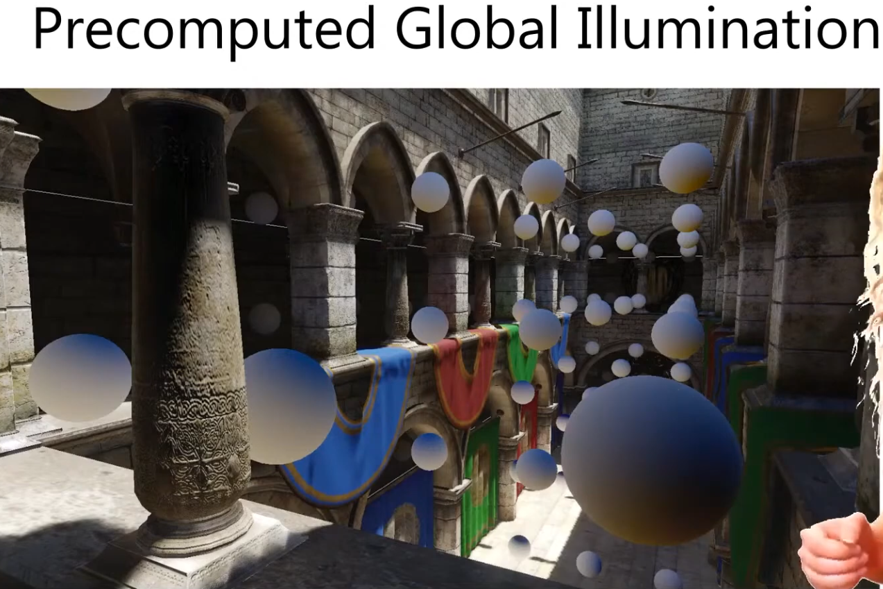 .
.
-
It doesn't matter what method we use for computing the GI.
-
Access the data from a texture; trilinear filter it and we are done.
-
Easy and cheap.
-
Only works for static scenes.
Light Maps
-
 .
.
-
 .
.
-
-
-
See the source in VSCode.
-
-
Limitations :
-
Specularity changes based on the angle of the camera, so it cannot be baked into the geometry; this is view dependent.
-
No specular indirect lighting baked.
-
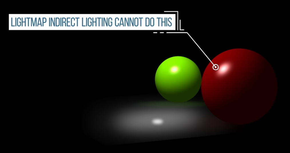 .
.
-
Light Bleeding
-
Fixing light bleeding in Lightmaps - Unity .
-
Solutions :
-
If you provide lightmap UVs yourself, add margins using your modeling package.
-
~If Unity automatically generates the lightmap UVs for a Model, you can tell Unity to increase the pack margin. Bla bla bla.
-
Increase the resolution:
-
Of the entire lightmap. This will increase the number of pixels between the charts and therefore reduce the likelihood of bleeding. The downside is that your lightmap may become too large.
-
Of a single GameObject. This allows you to increase lightmap resolution only for GameObjects that have overlapping UVs. Though less likely, this can also increase your lightmap size.
-
-
I believe what Unity means is:
-
It must use a different texture for lightmaps, overlaid on top of the albedo.
-
Therefore, it makes sense to talk about "increasing the lightmap resolution" since it's a separate texture.
-
-
-
-
Aliasing on UV Seams - Adobe .
-
Solutions :
-
Increase the output texture resolution of the Bakers.
-
Increase the Anti-aliasing setting (note: it may take more time to compute).
-
Align the UVs to the pixel grid in the UV editor of the 3D modeling software.
-
Give a better Texel Ratio to UVs.
-
-
-
My question :
-
Caio:
-
the light is baked in, so I guess it makes sense to be a UV issue, causing the texture bleeding
-
-
devsh:
-
 .
.
-
welcome to the fundamental problem with lightmapping
-
Pixar solves it with PTEX .
-
"Per-Face Texture Mapping for Production Rendering".
-
-
as a mere mortal you need to clamp the max mip level, anisotropy, and add padding texels around every UV island
-
you may also want to adjust the way you island your faces
-
-
Caio:
-
Interesting, I've never heard of this. I'm not using mipmap nor AA for now, I'm still setting things up
-
-
Devsh:
-
well then it's bilinear interpolation bleed
-
your pixel centers are not on the edge, there are no padding/border pixels.
-
-
Caio:
-
so it's not a problem with the UVs?
-
I'm a bit confused, is this fixed by implementing AA or mipmap?
-
-
Devsh:
-
no, it's made worse by mip-mapping
-
-
Caio:
-
so, from what I'm seeing, this is caused when generating the lightmap and baking the light color into the albedo texture? The lack of padding or UV overlap, etc. So, from what I'm understanding, this isn't caused by some oversight on my part, but this is an external issue that my render engine could fix at runtime? You said something about "bilinear interpolation bleed" "clamp the max mip level, anisotropy and add padding texels around every UV island", so I got confused about who's to blame for the artifact, my rendering engine or external software used to generate the lightmap?
-
-
Devsh:
-
both, you need to generate the input data better, and your engine needs to take care not to accidentally enable mip-mapping later on
-
-
Caio:
-
just a final clarification: are you considering that the lightmap is from a separate texture from the albedo, or the light is baked into the albedo? This is a free model, I didn't make the light baking myself. So when you say "generate the input data better", are you referring to the texture the light was baked into, or some other "input"? Finally, if it is the case that I can't rebake the texture, is there something I can do to reduce the artifact, or are all my options just to keep it from getting worse with mipmapping?
-
-
Post-Processing
Color Spaces, HDR / SDR, ToneMapping, Exposure
Color Spaces
Linear
vec3 srgb_to_linear_approx(vec3 srgb) {
    return pow(srgb, vec3(2.2));
}

vec3 linear_to_srgb_approx(vec3 linear) {
    return pow(linear, vec3(1.0 / 2.2));
}
vec3 linear_to_srgb(vec3 color) {
    //if going to srgb, clamp from 0 to 1.
    color = clamp(color, vec3(0.0), vec3(1.0));
    const vec3 a = vec3(0.055f);
    return mix((vec3(1.0f) + a) * pow(color.rgb, vec3(1.0f / 2.4f)) - a, 12.92f * color.rgb, lessThan(color.rgb, vec3(0.0031308f)));
}


vec3 srgb_to_linear(vec3 srgb) {
    vec3 cutoff = step(vec3(0.04045), srgb);
    vec3 low    = srgb / 12.92;
    vec3 high   = pow((srgb + 0.055) / 1.055, vec3(2.4));
    return mix(low, high, cutoff);
}

vec3 linear_to_srgb(vec3 linear) {
    vec3 cutoff = step(vec3(0.0031308), linear);
    vec3 low  = linear * 12.92;
    vec3 high  = pow(linear, vec3(1.0/2.4)) * 1.055 - 0.055;
    return mix(low, high, cutoff);
}
HDR, SDR, LDR
-
The word dynamic refers to the range of luminance (brightness) values that can be represented and displayed — from the darkest blacks to the brightest highlights.
-
HDR (High Dynamic Range):
-
A standard that represents a wide range of brightness and color, preserving details in both dark and bright areas.
-
Brightness :
-
Can reach 600–2000+ nits depending on the display, allowing much brighter highlights.
-
-
Color Gamut :
-
Often uses Rec.2020 or DCI-P3, covering a wider range of colors.
-
-
Formats :
-
Multiple formats exist (HDR10, HDR10+, Dolby Vision, HLG), requiring display and content compatibility.
-
-
-
SDR (Standard Dynamic Range):
-
The traditional display standard with limited brightness and color range, typically around 100 nits and Rec.709 gamut.
-
Brightness :
-
Typically limited to around 100 nits peak brightness.
-
-
Color Gamut :
-
Typically uses Rec.709 color space (sRGB).
-
-
Formats :
-
Standardized and widely compatible, but visually limited.
-
-
LDR (Low Dynamic Range):
-
A more generic term for images or rendering with restricted tonal range, often limited to 8-bit precision and prone to clipping in highlights and shadows.
-
All LDR fits inside SDR; it's an informal subset.
-
-
-
 .
.
-
 .
.
-
Exposure
-
In most rendering pipelines, exposure is applied as a simple scalar multiplier on the scene-linear color:
-
color_exposed = color_linear * k
-
-
where
kis some gain factor. -
Many engines define
krelative to an exposure offset in stops (like in photography). Each stop corresponds to doubling or halving the light. -
For example:
color *= exp2(ev);-
ev= exposure value in stops. -
exp2(ev)= $2^{ev}$. -
ev = +1.0→ multiply color by 2 (one stop brighter). -
ev = -1.0→ multiply color by 0.5 (one stop darker). -
ev = 0.0→ multiply by 1 (no change).
-
-
See https://google.github.io/filament/Filament.md.html#imagingpipeline/physicallybasedcamera for more information.
// Computes the camera's EV100 from exposure settings
// aperture in f-stops
// shutterSpeed in seconds
// sensitivity in ISO
float exposureSettings(float aperture, float shutterSpeed, float sensitivity) {
    return log2((aperture * aperture) / shutterSpeed * 100.0 / sensitivity);
}

// Computes the exposure normalization factor from
// the camera's EV100
float exposure(float ev100) {
    return 1.0 / (pow(2.0, ev100) * 1.2);
}

float ev100 = exposureSettings(aperture, shutterSpeed, sensitivity);
float exposure = exposure(ev100);

vec4 color = evaluateLighting();
color.rgb *= exposure;
-
Example :
-
Material
-
Base color: sRGB 0.81, 0, 0
-
Metallic: 0
-
Roughness: 0
-
Reflectance: 0.5
-
-
Indirect light: IBL
-
256×256 cubemap generated by cmgen from office.exr
-
Multiplier: 35,000
-
-
Direct light: directional light
-
Linear color: 1.0, 0.96, 0.95
-
Intensity: 120,000 lux
-
-
Exposure
-
Aperture: f/16
-
Shutter speed: 1/125s
-
ISO: 100
-
-
 .
.
-
Tone Mapping
-
Filament: Perform post-processing on the scene-referred data (linear space, before tone-mapping) as much as possible.
-
Range Compression :
-
Convert HDR luminance to LDR luminance.
-
-
Color Space Conversion :
-
Convert LDR luminance to the desired color space (RGB, XYZ, CMYK, etc).
-
-
Baked as LUT :
-
“Bakes” the transform:
-
3D LUT:
-
Encodes the full color mapping (linear → display).
-
-
1D LUTs:
-
Sometimes used for individual transfer functions (e.g., gamma, log encoding).
-
-
This is less flexible (changing exposure or dynamic response means regenerating the LUT) but can be faster or simpler.
-
This allows both dynamic range compression and color grading in one lookup.
-
Common in offline workflows (film, photography), less common in real-time engines because:
-
Needs large 3D textures for precision.
-
Harder to tweak exposure/gamma without regenerating the LUT.
-
-
-
ACES :
-
Industry-standard color pipeline used in film/VFX.
-
ACES defines a full rendering pipeline:
-
Input color space conversion (scene-linear → ACEScg).
-
Rendering transform (RRT).
-
Output transform (ODT) for the target display (sRGB, Rec.709, HDR10, etc.).
-
The ODT contains the tone mapping curve that compresses HDR highlights, so the final result isn’t “blown out.”
-
-
-
If you’re implementing “ACES without LUT” and using the standard analytical approximation (often seen in game engines, e.g. the Narkowicz ACES fit), you are applying that curve. That’s why your results look controlled.
-
Core includes a tone-mapping-like step in the RRT+ODT chain.
-
The ACES RRT+ODT math is the “recipe.” If you would bake this into a LUT, the LUT would be a “pre-baked version of the recipe” so software can apply it quickly without recalculating everything.
-
-
AgX :
-
AgX .
-
AgX without LUT
-
You’re skipping its actual rendering transform, so you’re just doing a color space conversion, not a tonemap.
-
-
AgX is normally delivered and used as a full view transform (shaper + contrast + color transforms) in OCIO configs and as pre-baked LUTs.
-
A more recent open-source rendering transform for 3D (often seen in Blender).
-
Similar idea to ACES: a defined rendering transform that compresses HDR → display space with filmic-like contrast.
-
AgX is newer and designed around filmic contrast with a wider shoulder/roll-off.
-
The official AgX distribution is often provided as LUTs (for Blender, Nuke, etc.).
-
If you apply only the matrix transforms (input → working space → output primaries) but skip the LUT (the part that encodes the log-like shaper + contrast mapping), you’re basically just viewing scene-linear → display without the tonemapping curve.
-
Result: very bright, blown-out highlights.
-
-
Luminance visualization for debug :
-
Implementation of a custom debug tone-mapping operator for luminance visualization:
vec3 Tonemap_DisplayRange(const vec3 x) { // The 5th color in the array (cyan) represents middle gray (18%) // Every stop above or below middle gray causes a color shift float v = log2(luminance(x) / 0.18); v = clamp(v + 5.0, 0.0, 15.0); int index = int(floor(v)); return mix(debugColors[index], debugColors[min(15, index + 1)], fract(v)); } const vec3 debugColors[16] = vec3[]( vec3(0.0, 0.0, 0.0), // black vec3(0.0, 0.0, 0.1647), // darkest blue vec3(0.0, 0.0, 0.3647), // darker blue vec3(0.0, 0.0, 0.6647), // dark blue vec3(0.0, 0.0, 0.9647), // blue vec3(0.0, 0.9255, 0.9255), // cyan vec3(0.0, 0.5647, 0.0), // dark green vec3(0.0, 0.7843, 0.0), // green vec3(1.0, 1.0, 0.0), // yellow vec3(0.90588, 0.75294, 0.0), // yellow-orange vec3(1.0, 0.5647, 0.0), // orange vec3(1.0, 0.0, 0.0), // bright red vec3(0.8392, 0.0, 0.0), // red vec3(1.0, 0.0, 1.0), // magenta vec3(0.6, 0.3333, 0.7882), // purple vec3(1.0, 1.0, 1.0) // white );-
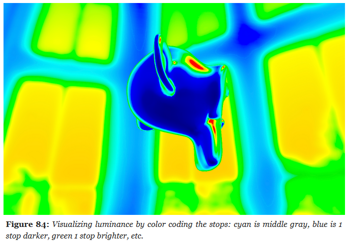 .
.
-
Bloom / Glow
-
-
The idea of levels is interesting, and the use of a Glow Map is very cool, giving a lens dirt look.
-
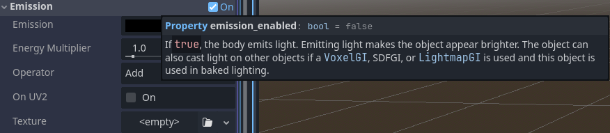 .
.
-
-
Filament Engine code:
vec4 surfaceShading() {
    vec4 color = evaluateLights();
    // rgb = color, w = exposure compensation
    vec4 emissive = getEmissive();
    color.rgb += emissive.rgb * pow(2.0, ev100 + emissive.w - 3.0);
    color.rgb *= exposure;
    return color;
}
-
ChatGPT code, I think:
// Note: FBO is FrameBuffer Object (Color Attachment).

// Bright-pass fragment shader (extract bright areas)
#version 330 core
in vec2 vUV;
out vec4 FragColor;

uniform sampler2D sceneTex;    // HDR scene texture (RGB, float)
uniform float threshold;       // brightness threshold
uniform float knee;            // soft knee (0..1). 0 = hard threshold

// Convert RGB luminance (sRGB or linear - be consistent with your pipeline)
float luminance(vec3 c) {
    // If your sceneTex is linear, use linear luminance.
    return dot(c, vec3(0.2126, 0.7152, 0.0722));
}

void main() {
    vec3 color = texture(sceneTex, vUV).rgb;
    float l = luminance(color);

    // smooth threshold (Reinhard-style soft knee)
    float t = threshold;
    float k = knee * t;
    float soft = clamp((l - (t - k)) / (k + 1e-6), 0.0, 1.0);
    float contribution = max(l - t, 0.0) / (max(l, 1e-6)) ; // preserves color hue for very bright
    // Blend soft and hard:
    float mask = max(contribution, soft);

    FragColor = vec4(color * mask, 1.0);
}

// Separable Gaussian blur fragment shader (use twice: horizontal then vertical)
#version 330 core
in vec2 vUV;
out vec4 FragColor;

uniform sampler2D image;
uniform vec2 texelSize;   // 1.0 / textureSize (width, height)
uniform vec2 direction;   // (1,0) horizontal pass, (0,1) vertical pass

// 9-tap Gaussian weights (can be adjusted). Symmetric kernel.
const float weights[9] = float[](
    0.051, 0.0918, 0.12245, 0.1531, 0.1633, 0.1531, 0.12245, 0.0918, 0.051
);

void main() {
    vec3 result = vec3(0.0);
    // center tap
    result += texture(image, vUV).rgb * weights[4];

    // sample pairs
    for (int i = 1; i <= 4; ++i) {
        vec2 offset = direction * texelSize * float(i);
        vec3 t1 = texture(image, vUV + offset).rgb;
        vec3 t2 = texture(image, vUV - offset).rgb;
        float w = weights[4 + i]; // symmetric indexing where center is index 4
        // weights array arranged so index maps: 0..8 with center at 4
        result += (t1 + t2) * w;
    }

    FragColor = vec4(result, 1.0);
}

// Composite fragment shader (add bloom to scene + optional tonemapping)
#version 330 core
in vec2 vUV;
out vec4 FragColor;

uniform sampler2D sceneTex;   // original HDR scene (no bright-pass)
uniform sampler2D bloomTex;   // blurred bright-pass
uniform float bloomIntensity; // how much bloom to add
uniform float exposure;       // optional exposure for tonemapping
uniform bool  applyTonemap;   // whether to apply simple tonemap

vec3 acesFilm(vec3 x) {
    // small ACES tone curve approximation (optional)
    const float a = 2.51;
    const float b = 0.03;
    const float c = 2.43;
    const float d = 0.59;
    const float e = 0.14;
    return clamp((x*(a*x+b))/(x*(c*x+d)+e), 0.0, 1.0);
}

void main() {
    vec3 hdr = texture(sceneTex, vUV).rgb;
    vec3 bloom = texture(bloomTex, vUV).rgb;

    vec3 combined = hdr + bloom * bloomIntensity;

    vec3 mapped = combined;
    if (applyTonemap) {
        mapped = acesFilm(combined * exposure);
    } else {
        // simple exposure clamp
        mapped = 1.0 - exp(-combined * exposure);
    }

    FragColor = vec4(mapped, 1.0);
}
Etc
LUT (Look Up Table)
-
Applies a color transformation by remapping colors according to a precomputed table. Usually for grading, stylization, or fine-tuned color correction.
-
Takes already tonemapped LDR (or sometimes linear HDR) colors and remaps them for a particular “look.”
-
1D LUT :
-
Adjusts a single channel independently (e.g., gamma, exposure).
-
-
3D LUT :
-
Remaps full RGB triples (commonly used in film and games for grading).
-
-
Format :
-
.cube -
.png
-
-
Godot LUT Applying :
vec3 apply_bcs(vec3 color, vec3 bcs) {
    color = mix(vec3(0.0f), color, bcs.x);
    color = mix(vec3(0.5f), color, bcs.y);
    color = mix(vec3(dot(vec3(1.0f), color) * 0.33333f), color, bcs.z);
    return color;
}

#ifdef USE_1D_LUT
vec3 apply_color_correction(vec3 color) {
    color.r = texture(source_color_correction, vec2(color.r, 0.0f)).r;
    color.g = texture(source_color_correction, vec2(color.g, 0.0f)).g;
    color.b = texture(source_color_correction, vec2(color.b, 0.0f)).b;
    return color;
}
#else
vec3 apply_color_correction(vec3 color) {
    return textureLod(source_color_correction, color, 0.0).rgb;
}
#endif
-
LUT Generation :
-
Code of
genbrdflut.vertandgenbrdflut.frag.
// Vertex Shader #version 450 layout (location = 0) out vec2 outUV; void main() { outUV = vec2((gl_VertexIndex << 1) & 2, gl_VertexIndex & 2); gl_Position = vec4(outUV * 2.0f - 1.0f, 0.0f, 1.0f); } // Frag Shader #version 450 layout (location = 0) in vec2 inUV; layout (location = 0) out vec4 outColor; layout (constant_id = 0) const uint NUM_SAMPLES = 1024u; const float PI = 3.1415926536; // Based omn http://byteblacksmith.com/improvements-to-the-canonical-one-liner-glsl-rand-for-opengl-es-2-0/ float random(vec2 co) { float a = 12.9898; float b = 78.233; float c = 43758.5453; float dt= dot(co.xy ,vec2(a,b)); float sn= mod(dt,3.14); return fract(sin(sn) * c); } vec2 hammersley2d(uint i, uint N) { // Radical inverse based on http://holger.dammertz.org/stuff/notes_HammersleyOnHemisphere.html uint bits = (i << 16u) | (i >> 16u); bits = ((bits & 0x55555555u) << 1u) | ((bits & 0xAAAAAAAAu) >> 1u); bits = ((bits & 0x33333333u) << 2u) | ((bits & 0xCCCCCCCCu) >> 2u); bits = ((bits & 0x0F0F0F0Fu) << 4u) | ((bits & 0xF0F0F0F0u) >> 4u); bits = ((bits & 0x00FF00FFu) << 8u) | ((bits & 0xFF00FF00u) >> 8u); float rdi = float(bits) * 2.3283064365386963e-10; return vec2(float(i) /float(N), rdi); } // Based on http://blog.selfshadow.com/publications/s2013-shading-course/karis/s2013_pbs_epic_slides.pdf vec3 importanceSample_GGX(vec2 Xi, float roughness, vec3 normal) { // Maps a 2D point to a hemisphere with spread based on roughness float alpha = roughness * roughness; float phi = 2.0 * PI * Xi.x + random(normal.xz) * 0.1; float cosTheta = sqrt((1.0 - Xi.y) / (1.0 + (alpha*alpha - 1.0) * Xi.y)); float sinTheta = sqrt(1.0 - cosTheta * cosTheta); vec3 H = vec3(sinTheta * cos(phi), sinTheta * sin(phi), cosTheta); // Tangent space vec3 up = abs(normal.z) < 0.999 ? vec3(0.0, 0.0, 1.0) : vec3(1.0, 0.0, 0.0); vec3 tangentX = normalize(cross(up, normal)); vec3 tangentY = normalize(cross(normal, tangentX)); // Convert to world Space return normalize(tangentX * H.x + tangentY * H.y + normal * H.z); } // Geometric Shadowing function float G_SchlicksmithGGX(float dotNL, float dotNV, float roughness) { float k = (roughness * roughness) / 2.0; float GL = dotNL / (dotNL * (1.0 - k) + k); float GV = dotNV / (dotNV * (1.0 - k) + k); return GL * GV; } vec2 BRDF(float NoV, float roughness) { // Normal always points along z-axis for the 2D lookup const vec3 N = vec3(0.0, 0.0, 1.0); vec3 V = vec3(sqrt(1.0 - NoV*NoV), 0.0, NoV); vec2 LUT = vec2(0.0); for(uint i = 0u; i < NUM_SAMPLES; i++) { vec2 Xi = hammersley2d(i, NUM_SAMPLES); vec3 H = importanceSample_GGX(Xi, roughness, N); vec3 L = 2.0 * dot(V, H) * H - V; float dotNL = max(dot(N, L), 0.0); float dotNV = max(dot(N, V), 0.0); float dotVH = max(dot(V, H), 0.0); float dotNH = max(dot(H, N), 0.0); if (dotNL > 0.0) { float G = G_SchlicksmithGGX(dotNL, dotNV, roughness); float G_Vis = (G * dotVH) / (dotNH * dotNV); float Fc = pow(1.0 - dotVH, 5.0); LUT += vec2((1.0 - Fc) * G_Vis, Fc * G_Vis); } } return LUT / float(NUM_SAMPLES); } void main() { outColor = vec4(BRDF(inUV.s, 1.0-inUV.t), 0.0, 1.0); } -
Brightness, Contrast, Saturation (BCS)
-
Brightness, Contrast, Saturation :
-
bcs.x→ brightness/contrast scaling (closer to contrast, but with black reference). -
bcs.y→ bias toward mid-gray (brightness adjustment). -
bcs.z→ saturation (grayscale ↔ color).
-
// GODOT
vec3 apply_bcs(vec3 color, vec3 bcs) {
    color = mix(vec3(0.0f), color, bcs.x);
    color = mix(vec3(0.5f), color, bcs.y);
    color = mix(vec3(dot(vec3(1.0f), color) * 0.33333f), color, bcs.z);
    return color;
}
Anti-Aliasing
DLAA / DLSS
-
Deep learning approaches.
-
Use dedicated HW (tensor cores) for learned reconstruction.
-
Can be used purely for AA (DLAA) or for upscaling+AA (DLSS).
-
Good quality but hardware- and driver-dependent.
-
Neural-network–based temporal method, no upscaling. Produces very high-quality AA, sharper than TAA, with excellent stability and minimal ghosting.
-
Limitation: only available on RTX-class GPUs with Tensor cores.
SMAA (Subpixel Morphological Anti-Aliasing)
-
Screen-space post-process filter.
-
Enhanced morphological approach with pattern detection and optional temporal/supersampling modes.
-
Better quality than FXAA for subpixel details.
-
Image-based edge detection + pattern matching + blending. Optional SMAA T2x (temporal) and SMAA 4x (spatial + temporal + supersampling) modes.
-
Pros:
-
Good quality / cost balance; preserves more detail than FXAA.
-
Preserves more detail than FXAA/MLAA.
-
Detects diagonal/subpixel edges better.
-
Simple to integrate (one or two passes).
-
Stable cost, doesn’t require motion vectors.
-
-
Cons:
-
Still a post-process (no true geometric sampling), optional temporal features add complexity.
-
Still a screen-space morphological filter: cannot fix shader aliasing or subpixel shimmering in motion.
-
Higher cost than FXAA but still lighter than MSAA/TAA.
-
Temporal variants (T2x, 4x) require history management, increasing complexity.
-
CMAA (Conservative Morphological Anti-Aliasing)
-
Screen-space post-process filter.
-
Lightweight post-process edge filter, designed as a cheaper alternative to SMAA/FXAA.
-
Its design goals are to be a better alternative to FXAA by:
-
Being minimally invasive so it can be acceptable as a replacement in a wide range of applications, including worst case scenarios such as text, repeating patterns, certain geometries (power lines, mesh fences, foliage), and moving images.
-
Running efficiently on low-medium range GPU hardware, such as integrated GPUs (or, in our case, mobile GPUs).
-
-
CMAA has four basic logical steps:
-
Image analysis for colour discontinuities (afterwards stored in a local compressed 'edge' buffer). The method used is not unique to CMAA.
-
Extracting locally dominant edges with a small kernel. (Unique variation of existing algorithms.)
-
Handling of simple shapes.
-
Handling of symmetrical long edge shapes. (Unique take on the original MLAA shape handling algorithm.)
-
-
Pros:
-
Very low GPU cost.
-
Preserves sharpness better than FXAA in many cases.
-
Good fit for low-power or bandwidth-limited platforms.
-
-
Cons:
-
Lower quality than SMAA (weaker on diagonal/subpixel edges).
-
No temporal stability; flickering/shimmering remains in motion.
-
Less widely adopted/documented compared to SMAA.
-
FXAA (Fast Approximate Anti-Aliasing)
-
Single-pass post-process edge detection + blur across edges. Very cheap.
-
Pros:
-
Minimal cost, easy to integrate.
-
-
Cons:
-
Blurs fine detail; cannot fix shader aliasing that is not visible as contrast edges.
-
TAA / TXAA (Temporal Anti-Aliasing)
-
TXAA is Nvidia’s branded temporal approach that combines MSAA + post filters.
-
Reduced motion blur, but has a lot of overall blur.
-
Jitter camera/sample positions per frame; blend current frame with reprojected history using motion vectors.
-
Pros:
-
Very effective at removing temporal shimmer and approximating supersampling without shading every sample.
-
-
Cons:
-
Requires motion vectors, depth history, good stationary/visibility rejection; can cause ghosting and blur; tuning is scene- and engine-dependent.
-
-
Opinions :
-
Playing some modern games can be really fatiguing because TAA makes things look just out-of-focus enough to find myself reflexively squinting at them, which ain't great for eye-health.
-
MSAA (Multisample Anti-Aliasing)
-
Multiple coverage samples per pixel calculated during rasterization; shading can be either per-sample or per-pixel depending on pipeline settings.
-
Pros:
-
Correct geometric edge AA, stable across frames, no history artifacts.
-
-
Cons:
-
Multiplies memory bandwidth and (potentially) fragment-shading cost.
-
Poor fit for deferred shading unless you maintain multisampled G-buffers or use expensive workarounds.
-
-
-
Cool.
-
-
Advanced video on the subject .
-
I don't like this guy AT ALL, omfg.
-
MFAA (Multi-Frame Sampled Anti-Aliasing)
-
Driver/GPU alternates sample patterns across frames and accumulates to approximate higher-sample MSAA cheaply. Driver-level, not always available.
-
Can achieve MSAA-like appearance at lower immediate cost, but depends on driver & GPU; not a universal solution for engine-level integration.
Light Path / Rendering Method
-
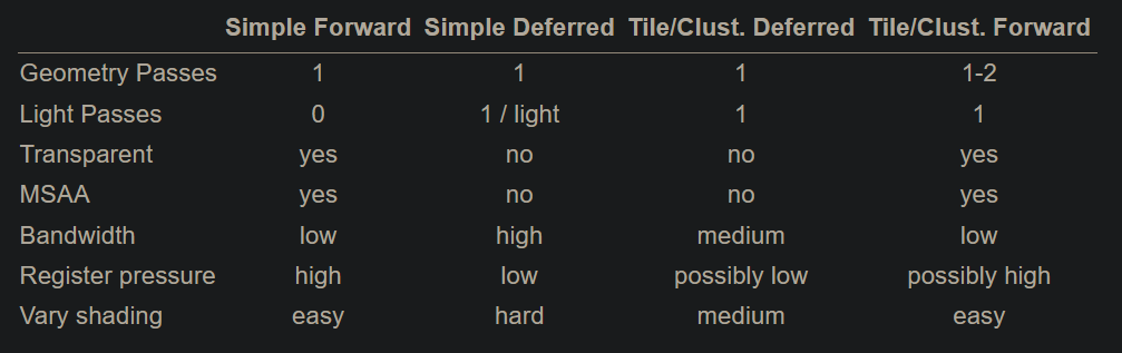 .
.
-
From the Real-Time Rendering 4th Edition.
-
-
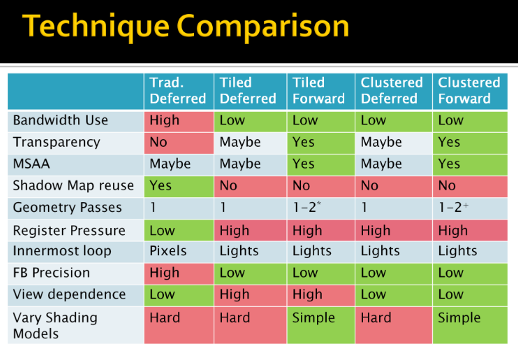 .
.
-
By Ola Olsson.
-
Forward Rendering
Forward
-
Geometry is shaded as it is drawn. For each triangle/pixel, the fragment shader loops over the lights that affect that object (or uses some per-object light set).
-
Lighting for a fragment is computed when that fragment is shaded, using the set of lights you feed to that draw call/shader.
-
Shading and output to the final render target happen in one pass.
-
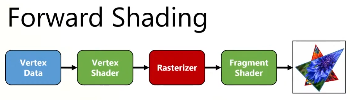 .
.
-
Overdraw happens, as the back triangle is shaded , but the front triangle overwrites the color on the screen.
-
-
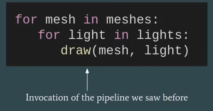 .
.
-
"Multipass forward rendering".
-
-
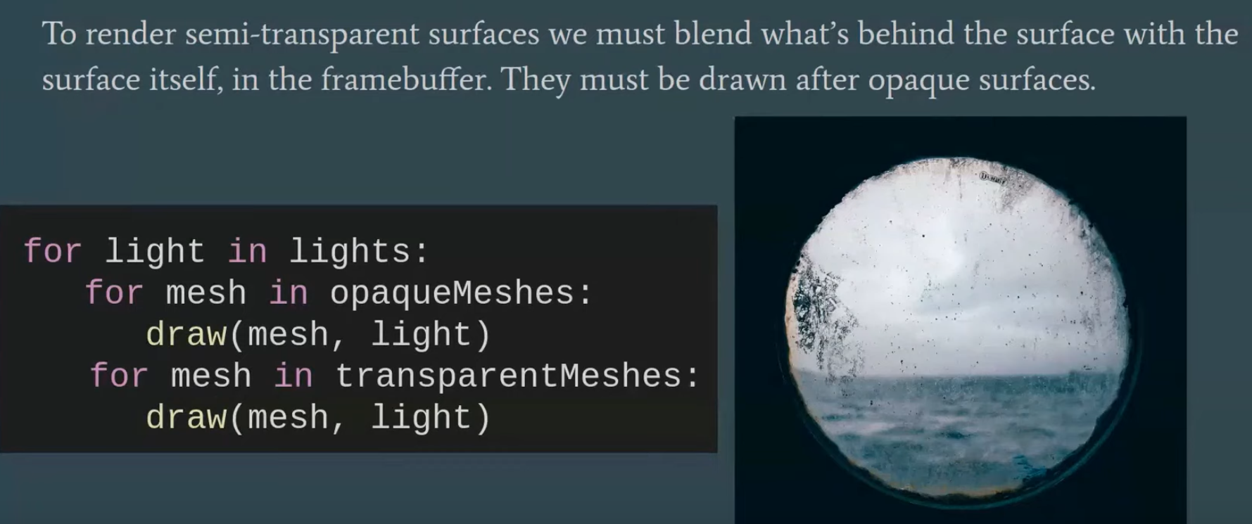 .
.
-
 .
.
Tiled Forward Shading
-
Tiled shading can be applied to both forward and deferred rendering methods.
-
The idea is to split the screen into a grid of tiles and, for each tile, find the list of lights that affect the pixels within that tile.
-
This has the advantage of reducing overdraw (in deferred rendering) and shading computations of large objects (in forward rendering).
-
However, this technique suffers from depth discontinuity issues that can lead to large amounts of extraneous work.
Gathering the lights
-
We now need to access all relevant lights for each pixel sequentially.
-
Just using a global list of lights is, of course, terribly inefficient.
-
On the other hand, creating lists of lights for each pixel individually is both slow and requires lots of storage.
-
Tiled shading strikes a balance, where we create lists for tiles of pixels.
-
The list must be conservative, storing all lights that may affect any sample within the tile.
-
So we trade some compute performance for bandwidth, which, as we have seen, is a good tradeoff on modern GPUs.
-
Each tile contains a single list of all the lights that might influence any of the pixels inside.
-
This list is shared between the pixels, so overhead for list maintenance and fetching is low.
Constructing the list
-
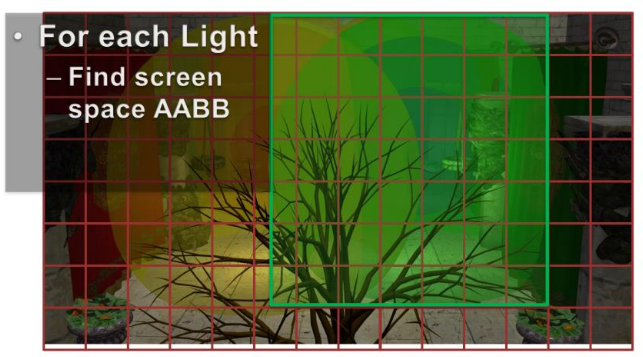
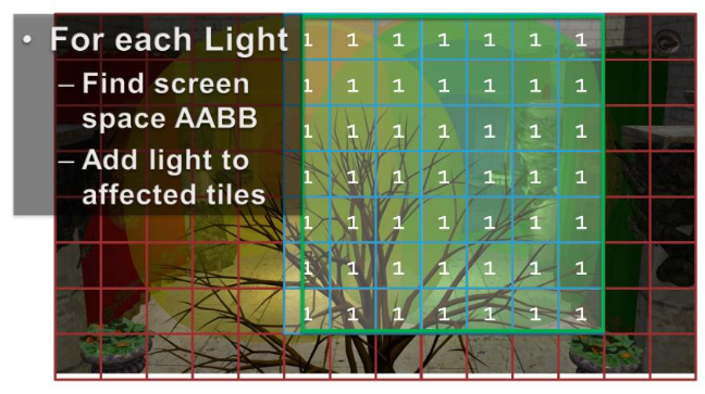
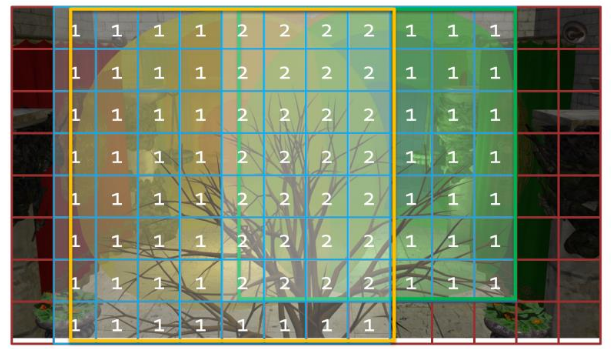 .
.
-
For each light, establish the screen space bounding box, illustrated for the green light.
-
Then add the index of the light to all overlapped tiles.
-
Then repeat this process for all remaining lights.
-
The illustration only shows the counts, so you need to imagine the lists being built as well.
-
In practice, we’d also do a conservative per-tile min/max depth test to cull away lights occupying empty space.
Vertex Shader
-
Vertex Output:
struct VertexShaderOutput { float3 positionVS : TEXCOORD0; // View space position. float2 texCoord : TEXCOORD1; // Texture coordinate float3 tangentVS : TANGENT; // View space tangent. float3 binormalVS : BINORMAL; // View space binormal. float3 normalVS : NORMAL; // View space normal. float4 position : SV_POSITION; // Clip space position. };-
I chose to do all of the lighting in view space, as opposed to world space, because it is easier to work in view space coordinates when implementing deferred shading and forward+ rendering techniques.
-
The
SV_POSITIONsemantic is applied to the output value from the vertex shader to specify that the value is used as the clip space position, but this semantic can also be applied to an input variable of a pixel shader. WhenSV_POSITIONis used as an input semantic to a pixel shader, the value is the position of the pixel in screen space. In both the deferred shading and the forward+ shaders, I will use this semantic to get the screen space position of the current pixel.
VertexShaderOutput VS_main( AppData IN ) { VertexShaderOutput OUT; OUT.position = mul( ModelViewProjection, float4( IN.position, 1.0f ) ); OUT.positionVS = mul( ModelView, float4( IN.position, 1.0f ) ).xyz; OUT.tangentVS = mul( ( float3x3 )ModelView, IN.tangent ); OUT.binormalVS = mul( ( float3x3 )ModelView, IN.binormal ); OUT.normalVS = mul( ( float3x3 )ModelView, IN.normal ); OUT.texCoord = IN.texCoord; return OUT; }-
You will notice that I am pre-multiplying the input vectors by the matrices. This indicates that the matrices are stored in column-major order by default.
-
Fragment Shader Inputs
-
Material :
-
Since some material properties can also have an associated texture (for example, diffuse textures, specular textures, or normal textures), we will also use the material to indicate if those textures are present on the object.
struct Material { float4 GlobalAmbient; //-------------------------- ( 16 bytes ) float4 AmbientColor; //-------------------------- ( 16 bytes ) float4 EmissiveColor; //-------------------------- ( 16 bytes ) float4 DiffuseColor; //-------------------------- ( 16 bytes ) float4 SpecularColor; //-------------------------- ( 16 bytes ) // Reflective value. float4 Reflectance; //-------------------------- ( 16 bytes ) float Opacity; float SpecularPower; // For transparent materials, IOR > 0. float IndexOfRefraction; bool HasAmbientTexture; //-------------------------- ( 16 bytes ) bool HasEmissiveTexture; bool HasDiffuseTexture; bool HasSpecularTexture; bool HasSpecularPowerTexture; //-------------------------- ( 16 bytes ) bool HasNormalTexture; bool HasBumpTexture; bool HasOpacityTexture; float BumpIntensity; //-------------------------- ( 16 bytes ) float SpecularScale; float AlphaThreshold; float2 Padding; //--------------------------- ( 16 bytes ) }; //--------------------------- ( 16 * 10 = 160 bytes )-
GlobalAmbient-
Describes the ambient contribution applied to all objects in the scene globally. Technically, this variable should be a global variable (not specific to a single object), but since there is only a single material at a time in the pixel shader, it’s fine to put it here.
-
-
Opacity-
Determines the total opacity of an object. This value can make objects appear transparent. This property is used to render semi-transparent objects in the transparent pass. If the opacity value is less than one (1 being fully opaque and 0 being fully transparent), the object is considered transparent and rendered in the transparent pass instead of the opaque pass.
-
-
SpecularPower-
Determines how shiny the object appears.
-
-
IndexOfRefraction-
Can be applied to objects that should refract light through them. Since refraction requires environment mapping techniques not implemented in this experiment, this variable will not be used here.
-
-
BumpIntensity-
If a model has a bump map, the material’s
HasBumpTextureproperty is set totrueand the model is bump-mapped instead of normal-mapped. -
Normal and bump maps are mutually exclusive, so they can reuse the same texture slot assignment.
-
-
SpecularScale-
Scales the specular power value read from a specular power texture. Since textures usually store values as unsigned normalized values, when sampling from the texture the value is read as a floating-point value in the range of
[0..1]. A specular power of 1.0 doesn’t make much sense, so the specular power value read from the texture will be scaled bySpecularScalebefore being used for the final lighting computation.
-
-
AlphaThreshold-
Can be used to discard pixels whose opacity is below a certain value using the “discard” command in the pixel shader. This is useful for “cut-out” materials where the object does not need alpha blending but should have holes (for example, a chain-link fence).
-
-
-
The material properties are passed to the pixel shader using a constant buffer.
cbuffer Material : register( b2 ) { Material Mat; }; Texture2D AmbientTexture : register( t0 ); Texture2D EmissiveTexture : register( t1 ); Texture2D DiffuseTexture : register( t2 ); Texture2D SpecularTexture : register( t3 ); Texture2D SpecularPowerTexture : register( t4 ); Texture2D NormalTexture : register( t5 ); Texture2D BumpTexture : register( t6 ); Texture2D OpacityTexture : register( t7 ); -
Lights :
StructuredBuffer<uint> LightIndexList: register( t9 ); Texture2D<uint2> LightGrid: register( t10 ); struct Light { /** * Position for point and spot lights (World space). */ float4 PositionWS; //--------------------------------------------------------------( 16 bytes ) /** * Direction for spot and directional lights (World space). */ float4 DirectionWS; //--------------------------------------------------------------( 16 bytes ) /** * Position for point and spot lights (View space). */ float4 PositionVS; //--------------------------------------------------------------( 16 bytes ) /** * Direction for spot and directional lights (View space). */ float4 DirectionVS; //--------------------------------------------------------------( 16 bytes ) /** * Color of the light. Diffuse and specular colors are not separated. */ float4 Color; //--------------------------------------------------------------( 16 bytes ) /** * The half angle of the spotlight cone. */ float SpotlightAngle; /** * The range of the light. */ float Range; /** * The intensity of the light. */ float Intensity; /** * Disable or enable the light. */ bool Enabled; //--------------------------------------------------------------( 16 bytes ) /** * Is the light selected in the editor? */ bool Selected; /** * The type of the light. */ uint Type; float2 Padding; //--------------------------------------------------------------( 16 bytes ) //--------------------------------------------------------------( 16 * 7 = 112 bytes ) };-
SpotlightAngle-
Is the half-angle of the spotlight cone expressed in degrees. Working in degrees is more intuitive than in radians. The spotlight angle is converted to radians in the shader when computing the cosine of the angle between the spotlight direction and the light vector.
-
-
Range-
For point lights, the range is the radius of the sphere that represents the light; for spotlights, it’s the length of the cone that represents the light. Directional lights don’t use range because they are considered infinitely far away, pointing in the same direction everywhere.
-
-
Intensity-
Modulates the computed light contribution. By default, this value is 1 but can make some lights brighter or dimmer than others.
-
-
Enabled-
Lights with
Enabledset tofalseare skipped in the shader.
-
-
Selected-
When a light is selected in the scene, its visual representation appears darker (less transparent) to indicate selection.
-
-
Type-
Can have one of the following values:
#define POINT_LIGHT 0 #define SPOT_LIGHT 1 #define DIRECTIONAL_LIGHT 2 -
-
Spot lights, point lights and directional lights are not separated into different structs and all of the properties necessary to define any of those light types are stored in a single struct.
-
The Position variable only applies to point and spot lights while the Direction variable only applies to spot and directional lights.
-
I store both world space and view space position and direction vectors because I find it easier to work in world space in the application then convert the world space vectors to view space before uploading the lights array to the GPU.
-
This way I do not need to maintain multiple light lists at the cost of additional space that is required on the GPU. But even 10,000 lights only require 1.12 MB on the GPU so I figured this was a reasonable sacrifice. But minimizing the size of the light structs could have a positive impact on caching on the GPU and improve rendering performance.
-
I chose not to separate the diffuse and specular color contributions because it is rare that these values differ.
-
The lights array is accessed through a StructuredBuffer . Most lighting shader implementations will use a constant buffer to store the lights array but constant buffers are limited to 64 KB in size which means that it would be limited to about 570 lights before running out of constant memory on the GPU. Structured buffers are stored in texture memory which is limited to the amount of texture memory available on the GPU (usually in the GB range on desktop GPUs). Texture memory is also very fast on most GPUs so storing the lights in a structured buffer did not impose a performance impact. In fact, on my particular GPU (NVIDIA GeForce GTX 680) I noticed a considerable performance improvement when I moved the lights array to a structure buffer.
StructuredBuffer<Light> Lights : register( t8 );
-
Fragment Shader
float3 ExpandNormal( float3 n )
{
    return n * 2.0f - 1.0f;
}

float4 DoNormalMapping( float3x3 TBN, Texture2D tex, sampler s, float2 uv )
{
    float3 normal = tex.Sample( s, uv ).xyz;
    normal = ExpandNormal( normal );

    // Transform normal from tangent space to view space.
    normal = mul( normal, TBN );
    return normalize( float4( normal, 0 ) );
}

float4 DoBumpMapping( float3x3 TBN, Texture2D tex, sampler s, float2 uv, float bumpScale )
{
    // Sample the heightmap at the current texture coordinate.
    float height = tex.Sample( s, uv ).r * bumpScale;
    // Sample the heightmap in the U texture coordinate direction.
    float heightU = tex.Sample( s, uv, int2( 1, 0 ) ).r * bumpScale;
    // Sample the heightmap in the V texture coordinate direction.
    float heightV = tex.Sample( s, uv, int2( 0, 1 ) ).r * bumpScale;

    float3 p = { 0, 0, height };
    float3 pU = { 1, 0, heightU };
    float3 pV = { 0, 1, heightV };

    // normal = tangent x bitangent
    float3 normal = cross( normalize(pU - p), normalize(pV - p) );

    // Transform normal from tangent space to view space.
    normal = mul( normal, TBN );

    return float4( normal, 0 );
}

float4 DoDiffuse( Light light, float4 L, float4 N )
{
    float NdotL = max( dot( N, L ), 0 );
    return light.Color * NdotL;
}

float4 DoSpecular( Light light, Material material, float4 V, float4 L, float4 N )
{
    float4 R = normalize( reflect( -L, N ) );
    float RdotV = max( dot( R, V ), 0 );

    return light.Color * pow( RdotV, material.SpecularPower );
}

// Compute the attenuation based on the range of the light.
float DoAttenuation( Light light, float d )
{
    return 1.0f - smoothstep( light.Range * 0.75f, light.Range, d );
}

LightingResult DoPointLight( Light light, Material mat, float4 V, float4 P, float4 N )
{
    LightingResult result;

    float4 L = light.PositionVS - P;
    float distance = length( L );
    L = L / distance;

    float attenuation = DoAttenuation( light, distance );

    result.Diffuse = DoDiffuse( light, L, N ) *
                      attenuation * light.Intensity;
    result.Specular = DoSpecular( light, mat, V, L, N ) *
                       attenuation * light.Intensity;

    return result;
}


float DoSpotCone( Light light, float4 L )
{
    // If the cosine angle of the light's direction
    // vector and the vector from the light source to the point being
    // shaded is less than minCos, then the spotlight contribution will be 0.
    float minCos = cos( radians( light.SpotlightAngle ) );
    // If the cosine angle of the light's direction vector
    // and the vector from the light source to the point being shaded
    // is greater than maxCos, then the spotlight contribution will be 1.
    float maxCos = lerp( minCos, 1, 0.5f );
    float cosAngle = dot( light.DirectionVS, -L );
    // Blend between the minimum and maximum cosine angles.
    return smoothstep( minCos, maxCos, cosAngle );
}

LightingResult DoSpotLight( Light light, Material mat, float4 V, float4 P, float4 N )
{
    LightingResult result;

    float4 L = light.PositionVS - P;
    float distance = length( L );
    L = L / distance;

    float attenuation = DoAttenuation( light, distance );
    float spotIntensity = DoSpotCone( light, L );

    result.Diffuse = DoDiffuse( light, L, N ) *
                       attenuation * spotIntensity * light.Intensity;
    result.Specular = DoSpecular( light, mat, V, L, N ) *
                       attenuation * spotIntensity * light.Intensity;

    return result;
}

LightingResult DoDirectionalLight( Light light, Material mat, float4 V, float4 P, float4 N )
{
    LightingResult result;

    float4 L = normalize( -light.DirectionVS );

    result.Diffuse = DoDiffuse( light, L, N ) * light.Intensity;
    result.Specular = DoSpecular( light, mat, V, L, N ) * light.Intensity;

    return result;
}


// This lighting result is returned by the
// lighting functions for each light type.
struct LightingResult
{
    float4 Diffuse;
    float4 Specular;
};

LightingResult DoLighting( StructuredBuffer<Light> lights, Material mat, float4 eyePos, float4 P, float4 N )
{
    float4 V = normalize( eyePos - P );

    LightingResult totalResult = (LightingResult)0;

    for ( int i = 0; i < NUM_LIGHTS; ++i )
    {
        LightingResult result = (LightingResult)0;

        // Skip lights that are not enabled.
        if ( !lights[i].Enabled ) continue;
        // Skip point and spot lights that are out of range of the point being shaded.
        if ( lights[i].Type != DIRECTIONAL_LIGHT &&
             length( lights[i].PositionVS - P ) > lights[i].Range ) continue;

        switch ( lights[i].Type )
        {
        case DIRECTIONAL_LIGHT:
        {
            result = DoDirectionalLight( lights[i], mat, V, P, N );
        }
        break;
        case POINT_LIGHT:
        {
            result = DoPointLight( lights[i], mat, V, P, N );
        }
        break;
        case SPOT_LIGHT:
        {
            result = DoSpotLight( lights[i], mat, V, P, N );
        }
        break;
        }
        totalResult.Diffuse += result.Diffuse;
        totalResult.Specular += result.Specular;
    }

    return totalResult;
}


[earlydepthstencil]
float4 PS_main( VertexShaderOutput IN ) : SV_TARGET
{
    // Everything is in view space.
    float4 eyePos = { 0, 0, 0, 1 };
    Material mat = Mat;

    // Diffuse
    float4 diffuse = mat.DiffuseColor;
    if ( mat.HasDiffuseTexture )
    {
        float4 diffuseTex = DiffuseTexture.Sample( LinearRepeatSampler, IN.texCoord );
        if ( any( diffuse.rgb ) )
        {
            diffuse *= diffuseTex;
        }
        else
        {
            diffuse = diffuseTex;
        }
    }

    // Opacity
    float alpha = diffuse.a;
    if ( mat.HasOpacityTexture )
    {
        // If the material has an opacity texture, use that to override the diffuse alpha.
        alpha = OpacityTexture.Sample( LinearRepeatSampler, IN.texCoord ).r;
    }

    // Ambient
    float4 ambient = mat.AmbientColor;
    if ( mat.HasAmbientTexture )
    {
        float4 ambientTex = AmbientTexture.Sample( LinearRepeatSampler, IN.texCoord );
        if ( any( ambient.rgb ) )
        {
            ambient *= ambientTex;
        }
        else
        {
            ambient = ambientTex;
        }
    }
    // Combine the global ambient term.
    ambient *= mat.GlobalAmbient;

    // Emissive
    float4 emissive = mat.EmissiveColor;
    if ( mat.HasEmissiveTexture )
    {
        float4 emissiveTex = EmissiveTexture.Sample( LinearRepeatSampler, IN.texCoord );
        if ( any( emissive.rgb ) )
        {
            emissive *= emissiveTex;
        }
        else
        {
            emissive = emissiveTex;
        }
    }

    // Specular
    if ( mat.HasSpecularPowerTexture )
    {
        mat.SpecularPower = SpecularPowerTexture.Sample( LinearRepeatSampler, IN.texCoord ).r \
                            * mat.SpecularScale;
    }

    // Normal mapping
    if ( mat.HasNormalTexture )
    {
        // For scenes with normal mapping, I don't have to invert the binormal.
        float3x3 TBN = float3x3( normalize( IN.tangentVS ),
                                 normalize( IN.binormalVS ),
                                 normalize( IN.normalVS ) );

        N = DoNormalMapping( TBN, NormalTexture, LinearRepeatSampler, IN.texCoord );
    }
    // Bump mapping
    else if ( mat.HasBumpTexture )
    {
        // For most scenes using bump mapping, I have to invert the binormal.
        float3x3 TBN = float3x3( normalize( IN.tangentVS ),
                                 normalize( -IN.binormalVS ),
                                 normalize( IN.normalVS ) );

        N = DoBumpMapping( TBN, BumpTexture, LinearRepeatSampler, IN.texCoord, mat.BumpIntensity );
    }
    // Just use the normal from the model.
    else
    {
        N = normalize( float4( IN.normalVS, 0 ) );
    }

    float4 P = float4( IN.positionVS, 1 );


    LightingResult lit = DoLighting( Lights, mat, eyePos, P, N );

    diffuse *= float4( lit.Diffuse.rgb, 1.0f ); // Discard the alpha value from the lighting calculations.

    float4 specular = 0;
    if ( mat.SpecularPower > 1.0f ) // If specular power is too low, don't use it.
    {
        specular = mat.SpecularColor;
        if ( mat.HasSpecularTexture )
        {
            float4 specularTex = SpecularTexture.Sample( LinearRepeatSampler, IN.texCoord );
            if ( any( specular.rgb ) )
            {
                specular *= specularTex;
            }
            else
            {
                specular = specularTex;
            }
        }
        specular *= lit.Specular;
    }

    // Get the index of the current pixel in the light grid.
    uint2 tileIndex = uint2( floor(IN.position.xy / BLOCK_SIZE) );

    // Get the start position and offset of the light in the light index list.
    uint startOffset = LightGrid[tileIndex].x;
    uint lightCount = LightGrid[tileIndex].y;

    LightingResult lit = (LightingResult)0; // DoLighting( Lights, mat, eyePos, P, N );

    for ( uint i = 0; i < lightCount; i++ )
    {
        uint lightIndex = LightIndexList[startOffset + i];
        Light light = Lights[lightIndex];

        LightingResult result = (LightingResult)0;

        switch ( light.Type )
        {
        case DIRECTIONAL_LIGHT:
        {
            result = DoDirectionalLight( light, mat, V, P, N );
        }
        break;
        case POINT_LIGHT:
        {
            result = DoPointLight( light, mat, V, P, N );
        }
        break;
        case SPOT_LIGHT:
        {
            result = DoSpotLight( light, mat, V, P, N );
        }
        break;
        }
        lit.Diffuse += result.Diffuse;
        lit.Specular += result.Specular;
    }

    diffuse *= float4( lit.Diffuse.rgb, 1.0f ); // Discard the alpha value from the lighting calculations.
    specular *= lit.Specular;

    return float4( ( ambient + emissive + diffuse + specular ).rgb, alpha * mat.Opacity );
}
-
EarlyDepthStencil :
-
The
[earlydepthstencil]attribute before the function indicates that the GPU should take advantage of early depth and stencil culling. This causes the depth/stencil tests to be performed before the pixel shader is executed. This attribute cannot be used on shaders that modify the pixel’s depth value by outputting a value using theSV_Depthsemantic. Since this pixel shader only outputs a color value using theSV_TARGETsemantic, it can take advantage of early depth/stencil testing to provide a performance improvement when a pixel is rejected. Most GPUs will perform early depth/stencil tests anyway even without this attribute, and adding this attribute to the pixel shader did not have a noticeable impact on performance, but I decided to keep the attribute anyway. -
Since all lighting computations are performed in view space, the eye position (the camera position) is always (0, 0, 0).
-
This is a nice side effect of working in view space: the camera’s eye position does not need to be passed as an additional parameter to the shader.
-
Cool.
-
-
-
First, we need to gather the material properties. If the material has textures associated with its various components, the textures will be sampled before the lighting is computed. After the material properties have been initialized, all the lights in the scene will be iterated, and the lighting contributions will be accumulated and modulated with the material properties to produce the final pixel color.
-
Comments :
-
Diffuse :
-
The
anyHLSL intrinsic function can be used to determine if any of the color components are non-zero. -
If the material also has a diffuse texture associated with it, then the color from the diffuse texture will be blended with the material’s diffuse color. If the material’s diffuse color is black (0, 0, 0, 0), then the material’s diffuse color will simply be replaced by the color in the diffuse texture.
-
-
Opacity :
-
By default, the fragment’s transparency value is determined by the alpha component of the diffuse color. If the material has an opacity texture associated with it, the red component of the opacity texture is used as the alpha value, overriding the alpha value in the diffuse texture. In most cases, opacity textures store only a single channel in the first component of the color returned from the Sample method. To read from a single-channel texture, we must read from the red channel, not the alpha channel. The alpha channel of a single-channel texture will always be 1, so reading the alpha channel from the opacity map (which is most likely a single-channel texture) would not provide the required value.
-
-
-
Lighting :
-
The lighting calculations for the forward rendering technique are performed in the
DoLightingfunction. This function accepts the following arguments:-
lights: The lights array (as a structured buffer) -
mat: The material properties that were just computed -
eyePos: The position of the camera in view space (which is always (0, 0, 0)) -
P: The position of the point being shaded in view space -
N: The normal of the point being shaded in view space
-
-
The view vector (
V) is computed from the eye position and the position of the shaded pixel in view space. -
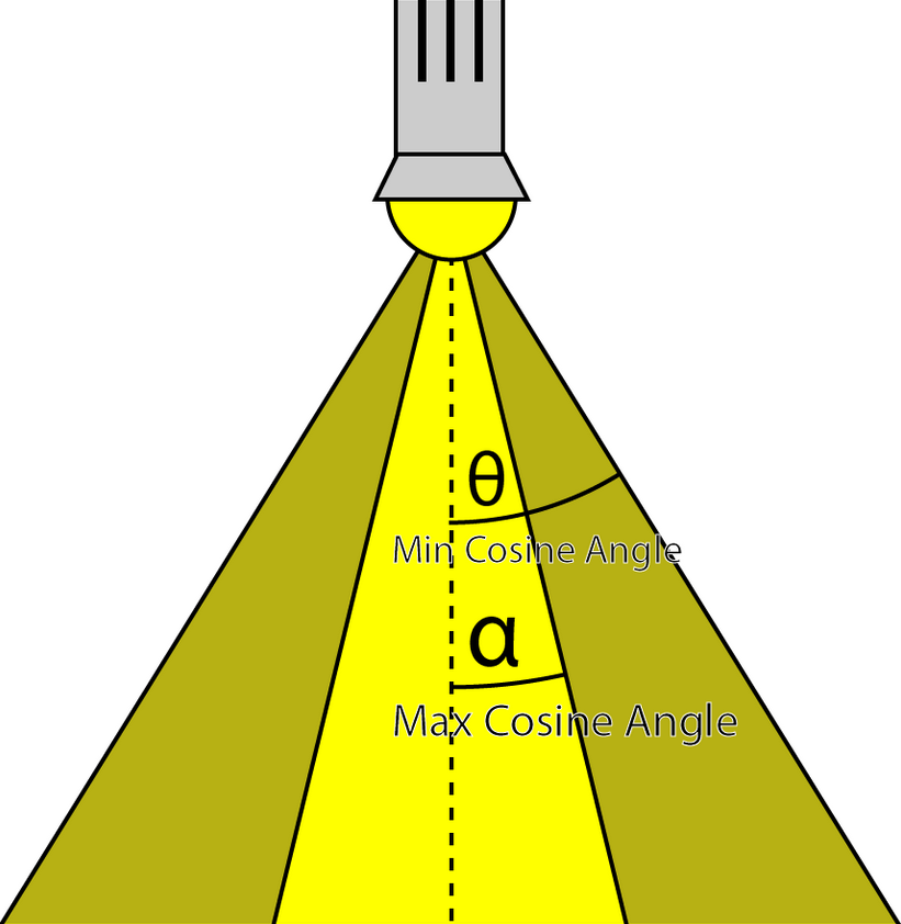 .
.
-
etc
-
Wicked Engine :
-
All the lights inside the camera are binned to small 8×8 pixel tiles on the screen. Each tile will thus have a minimal list of lights that should be iterated by every pixel inside when lighting up the surface.
-
The main optimizations I’ve used for some years now is the “2.5D culling” and the “flat bit arrays” methods, which I really liked.
-
I rearranged the light loops so they always operate strictly on one light type (directional/point/spot), which gave some minor performance improvement. So instead of one big loop that checks the type of light and calls the appropriate function, now there are 3 loops for each type. This also allowed to avoid all the tile checking for directional lights, because they are always affecting the full screen, that specific loop is just going over all of them which simplifies the shader further.
-
Visibility Buffer :
-
The main twist to the forward rendering is the inclusion of a secondary “visibility buffer”, to aid with effects that would better fit into a deferred renderer.
-
I always wanted to support all the post processing that deferred rendering supports, but normally forward rendering doesn’t write any G-Buffer textures to allow this. Some years ago I used a thin G-buffer for this written by the depth prepass.
-
Now the depth-prepass for the main camera writes a UINT texture that contains primitive IDs, this is called the visibility buffer.
-
This is some overhead compared to depth-only pass, but less than writing a G-buffer with multiple textures.
-
From this primitiveID texture any shader can get per-pixel information about any surface properties: depth, normal, roughness, velocity, etc.
-
The nice thing about it that we can get this on the async compute queue too, and that’s exactly what happens.
-
After the visibility buffer is completed in the prepass, the graphics queue continues rendering shadow maps, planar reflections and updating environment probes, while the compute queue starts working independently on rendering a G-buffer from the visibility buffer, but only if some effects are turned on that would require this:
-
depth buffer: it is always created from the visibility buffer. The normal depth buffer is always kept in depth write state, it’s never used as a sampled texture. This way the depth test efficiency remains the highest for the color and transparent passes later.
-
velocity: if any of the following effects are turned on: Temporal AA, Motion Blur, FSR upscaling, ray traced shadows/reflections/diffuse, SSR…
-
normal, roughness: if any of the following effects are turned on: SSR, ray traced reflections
-
some other params are simply retrieved from visibility buffer just on demand if effects need it, but not saved as a texture: for example face normal
-
light buffers: these are not separated, so things like blurred diffuse subsurface scattering is not supported. I support a simple wrapped and tinted NdotL term for subsurface scattering instead.
-
-
What does this texture actually store? It’s a single channel 32-bit UINT texture, and normally that wouldn’t be enough to store both primitive and instance ID. But there is a workaround, in which I store 25 bits of meshlet ID and 7 bits of primitive ID. A regular mesh wouldn’t fit into it, since it limits to 128 triangles, but with a lookup table it’s possible to manage.
-
-
Disadvantages
-
Tiled shading groups samples in rectangular screen-space tiles, using the min and max depth within each tile to define sub frustums. Thus, tiles which contain depth values that are close together, e.g. from a single surface, will be represented with small bounding volumes. However, for tiles where one or more depth discontinuities occur, the depth bounds of the tile must encompass all the empty space between the sample groups (illustrated in Figure 1). This reduces light culling efficiency, in the worst case degenerating to a pure 2D test. This results in a strong dependency between view and performance, which highly is undesirable in real-time applications, as it becomes difficult to guarantee consistent rendering performance at all times.
-
Visually, this means:
-
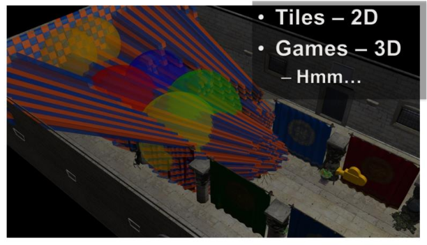 .
.
-
Toggling on the light geometry, we see that there is a lot of overlap, even in the empty space behind the tree.
-
We now should be able to start seeing the shape of the problem with 2D tiles in a 3D world.
-
 .
.
-
In 3D:
-
 .
.
-
While actually some of the samples, from the tree, are affected zero of these lights. While the tiger in the wall would only need two of the lights.
-
There is a fairly fundamental problem with tiled shading. The basic problem stems from that we are making the intersection between lights and geometry samples, both of which are 3D entities, in a 2D screen space.
-
The main practical issue with this is that the resulting light assignment is highly view dependent. This means that we cannot author scenes with any strong guarantee on performance, as a given view of the scene may have a significantly higher screen space light density than average.
-
For example, we’d like to be able to construct a scene with, say, maximum 4 lights affecting any part of the scene. In this case, we would like shading cost to be proportional to this, and stable, given different view points.
-
Unfortunately, no such correlation exists for tiled shading. In other words shading times are unpredictable, which is a major problem for a real time application.
-
Avalanche Studios :
-
The two tiled solutions need quite a bit of massaging to work reasonable well in all situations, especially with large amounts of depth discontinuities. There are proposed solutions that mitigate the problem, such as 2.5D culling, but they further complicate the code.
-
I didn’t have to go look for a problematic area, in fact, it was right there in front of my face. This shows how common these scenes actually are in real games, and certainly so in the games that we make.
-
 .
.
-
We are still using a deferred engine, but we could change to forward at any time should we decide that to be better. The important part is, however, that the transparency passes can now use the same lighting structure as the deferred passes, making it a unified lighting solution.
-
-
"Extensions to the Tiled Forward"
-
2.5D Culling :
-
2.5D Light Culling for Tiled Forward - Wicked Engine 2017 .
-
Depth discontinuity is the enemy of Forward+.
-
With a more aggressive culling we can eliminate false positives and have a much faster render.
-
-
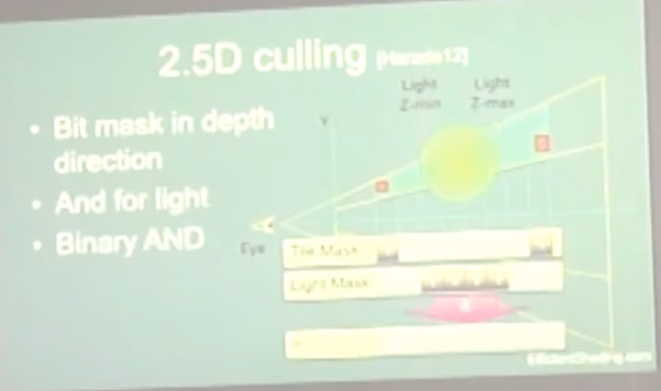 .
.
-
Avalanche Studios :
-
Criticizes the use of 2.5D Culling, considering that Cluster Shading yields a better result with less effort.
-
This is explained and demonstrated on pages 112 to 121 of this presentation: Efficient Real-Time Shading with Many Lights - Ola Olsson, Emil Persson (Avalanche) - 2014 .
-
2.5D Culling.
-
-
Bimodal Clusters / HalfZ :
-
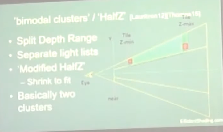 .
.
-
-
Ola Olsson:
-
This extensions have the problems of:
-
Lack of generality: slopes / multiple layers.
-
No solution for transparency.
-
Require depth pre-pass, as you have to work with the depth range to apply the extensions.
-
-
The use of Clustered Forward Shading removes the need for these extensions.
-
Samples
-
Forward, Deferred, Tile Forward Shading - DirectX11, HLSL - Sample - Jeremiah van Oosten 2024 .
-
There are 30,000,000,000 files, etc, C++, Visual Studio, CMake, etc. Jeebs.
-
The only relevant things are the shaders:
-
GraphicsTest\Assets\shaders\CommonInclude.hlsl -
GraphicsTest\Assets\shaders\ForwardPlusRendering.hlsl.
-
-
Papers and Presentations
-
Forward+: Bringing Deferred Lighting to the Next Level - AMD 2012 .
-
Forward, Deferred, Tiled Forward - Jeremiah Van Oosten - 2015 .
-
C++, shaders em HLSL.
-
Possui uma Sample acima.
-
-
Demo .
-
Demo .
-
Tiled Forward Shading vs Tiled Deferred Rendering - AMD 2013 (Jason Stewart and Gareth Thomas).-
The presentation is somewhat poor and the graphics are questionable.
-
No real-world lighting cases are presented.
-
"Have you looked into Forward Clustered?" Yea, but have not implemented, they are hours worth of work. I don't know if the extra complexity is worth, but I'll probably test it at some point.
-
They use Virtual Point Lights for GI, which sounds suspicious..
-
Clustered Forward Shading
-
Clustered shading expands on the idea of tiled rendering but adds a segmentation on the 3rd axis. The “clustering” is done in view space, by splitting the frustum into a 3D grid.
-
Clustered Shading enables using normal information to perform per-cluster back-face culling of lights, again reducing the number of lighting computations.
-
Clustered Shading vs Tiled Shading :
-
We also show that Clustered Shading not only outperforms tiled shading in many scenes, but also exhibits better worst case behaviour under tricky conditions (e.g. when looking at high-frequency geometry with large discontinuities in depth).
-
Additionally, Clustered Shading enables real-time scenes with two to three orders of magnitudes more lights than previously feasible (up to around one million light sources).
-
Our implementation shows much less view-dependent performance, and is much faster for some cases that are challenging for tiled shading.
-
Compared to tiled shading, clusters generally are smaller, and therefore will be affected by fewer light sources.
-
Our implementation shows that both clustered deferred and forward shading offer real-time performance and can scale up to 1M lights. In addition, overhead for the clustering is low, making it competitive even for few lights.
-
The shading cost is proportional to the light density.
-
-
Clustered Forward vs Clustered Deferred :
-
Clustered Shading is really decoupled from the choice between deferred or forward rendering. It works with both, so you’re not locked into one or the other. This way you can make an informed choice between the two approaches based on other factors, such as whether you need custom materials and lighting models, or need deferred effects such as screen-space decals, or simply based on performance.
-
Godot
-
Clustered lighting uses a compute shader to group lights into a 3D frustum aligned grid.
-
At render time, pixels can lookup what lights affect the grid cell they are in and only run light calculations for lights that might affect that pixel.
-
This approach can greatly speed up rendering performance on desktop hardware, but is substantially less efficient on mobile.
-
There's a default limit of 512 clustered elements that can be present in the current camera view.
-
A clustered element is an omni light, a spot light, a decal or a reflection probe.
-
This limit can be increased by adjusting Max Clustered Elements in Project Settings > Rendering > Limits > Cluster Builder.
-
High-level overview
-
Build the clustering data structure.
-
Render scene to Z Pre-pass.
-
Find visible clusters.
-
Reduce repeated values in the list of visible clusters.
-
Perform light culling and assign lights to clusters.
-
Shade samples using light list.
-
Steps two and six won’t be covered since they are mostly dependent on the shading model you’re using.
-
Steps three and four are combined into one and covered in the section on Determining Active Clusters, much like in Van Oosten’s implementation .
Building the Cluster Grid
-
Depth Slicing :
-
We’ll be focusing on building cluster grids that group samples based on their view space position. We’ll begin by tiling the view frustum exactly the same way you would in tiled shading and then subdividing it along the depth axis multiple times.
-
We choose to perform the subdivision in view space, by spacing the divisions exponentially to achieve self-similar subdivisions, such that the clusters become as cubical as possible (Figures 2(c) and 3).
-
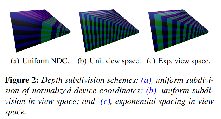
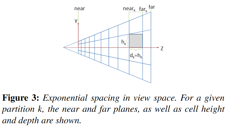 .
.
-
In Figure 3, we illustrate the subdivisions of a frustum. The number of subdivisions in the Y direction (Sy) is given in screen space (e.g. to form tiles of 32×32 pixels).
-
The near plane for a division k, near k, can be calculated from:
-
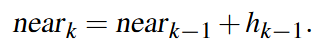 .
.
-
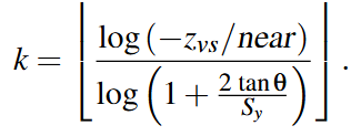 .
.
-
"I settled on a 16x9x24 subdivision because it matches my monitors aspect ratio, but it honestly could have been something else." - Angel Ortiz.
-
Doom (2016) :
-
Uses the one below, which doesn't represent any of the three above.
-
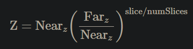 .
.
-
Solving:
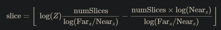 .
.
-
The major advantage of the equation above is that the only variable is Z and everything else is a constant.
-
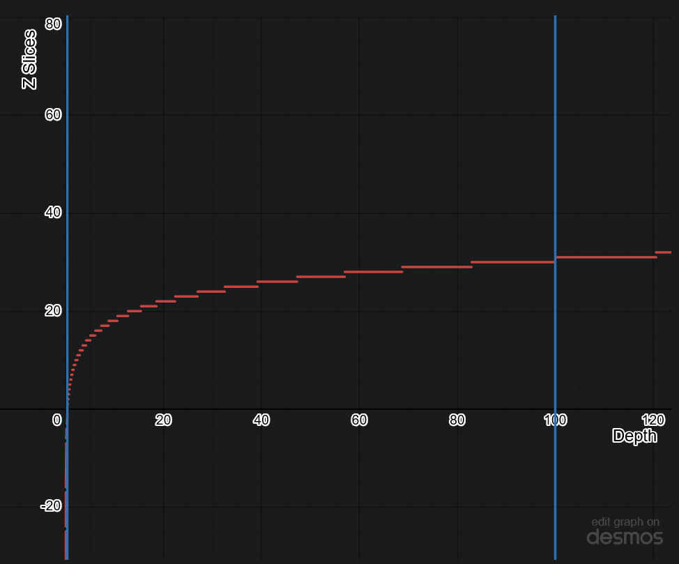 .
.
-
-
Avalanche Studios :
-
Another option we have considered, but not yet explored, is to not base it on pixel count, but simply divide the screen into a specific number of tiles regardless of resolution. This may reduce coherency on the GPU side somewhat in some cases, but would also decouple the CPU workload from the GPU workload and allow for some useful CPU side optimizations if the tile counts are known at compile time.
-
We are using exponential depth slicing, much like in the paper. There is nothing dictating that this is what we have to use, or for that matter that it is the best or most optimal depth slicing strategy; however, the advantage is that the shape of the clusters remain the same as we go deeper into the depth. On the other hand, clusters get larger in world space, which could potentially result in some distant clusters containing a much larger amount of lights. Depending on the game, it may be worth exploring other options.
-
Our biggest problem was that our depth ratio is massive, with near plane as close as 0.1m and far plane way out on the other side of the map, at 50,000m. This resulted in poor utilization of our limited depth slices, currently 16 of them. The step from one slice to the next is very large. Fortunately, in our game we don’t have any actual light sources beyond a distance of 500m. So we simply decided to keep our current distant light system for distances beyond 500m and limit the far range for clustering to that.
-
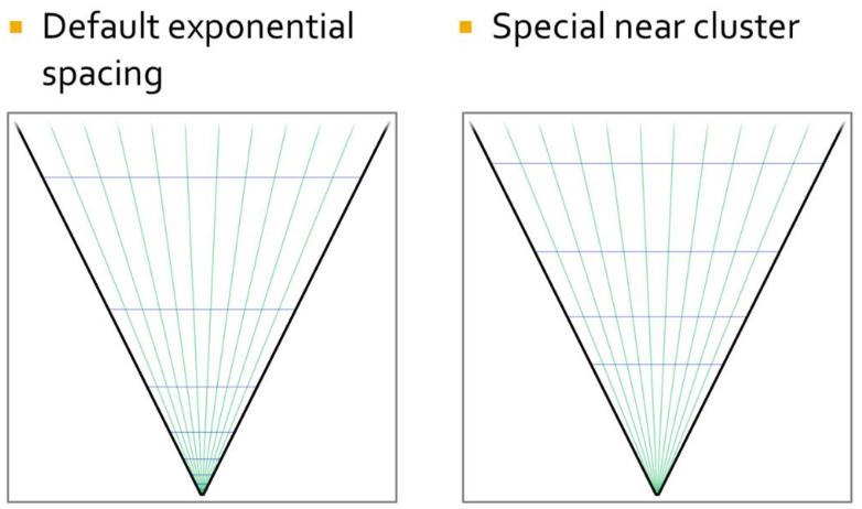 .
.
-
This improved the situation notably, but was still not ideal. We still burnt half of our slices on the first 7 meters from the camera. Given how our typical scenes look like, that’s likely going to be mostly empty space in most situations. So to improve the situation, we made the first slice special and made that go from near plane to an arbitrary visually tweaked distance, currently 5m. This gave us much better utilization.
-
-
Filament Engine :
-
The depth slicing is not linear, but exponential. In a typical scene, there will be more pixels close to the near plane than to the far plane. An exponential grid of froxels will therefore improve the assignment of lights where it matters the most.
-
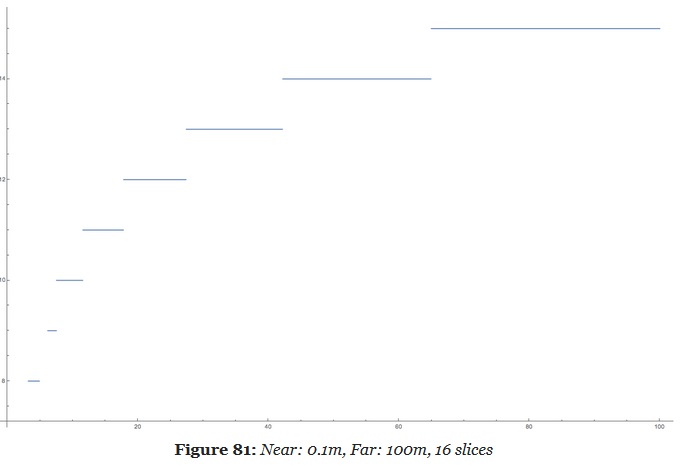 .
.
-
A simple exponential voxelization is unfortunately not enough. The graphic above clearly illustrates how world space is distributed across slices but it fails to show what happens close to the near plane.
-
A simple exponential distribution uses up half of the slices very close to the camera. In this particular case, we use 8 slices out of 16 in the first 5 meters. Since dynamic world lights are either point lights (spheres) or spot lights (cones), such a fine resolution is completely unnecessary so close to the near plane.
-
Our solution is to manually tweak the size of the first froxel depending on the scene and the near and far planes. By doing so, we can better distribute the remaining froxels across the frustum.
-
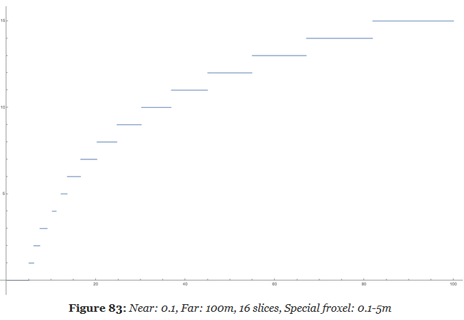 .
.
-
This new distribution is much more efficient and allows a better assignment of the lights throughout the entire frustum.
-
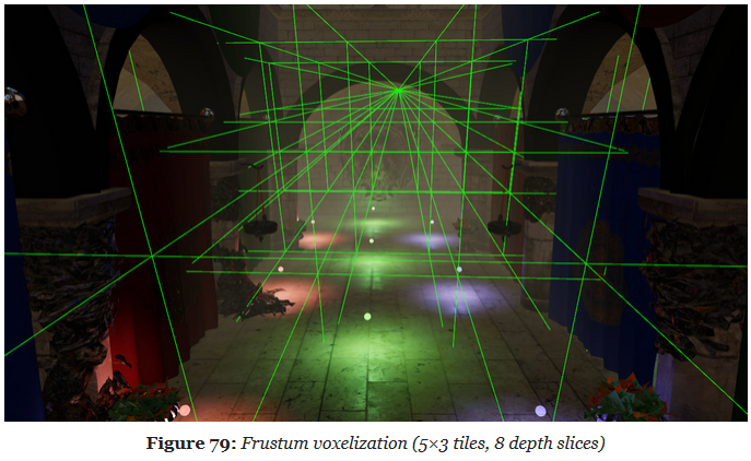
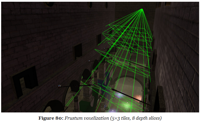
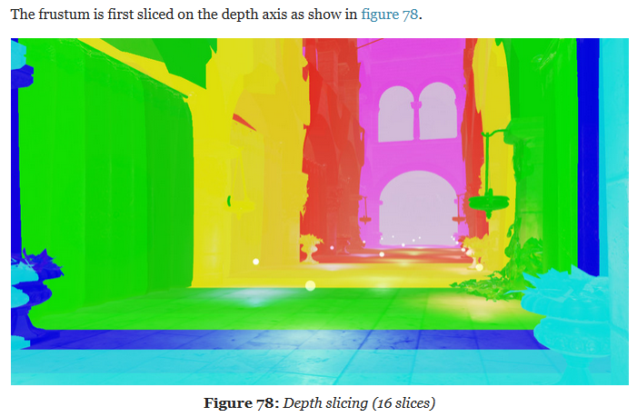 .
.
-
We call a froxel a voxel in frustum space.
-
The frustum voxelization can be executed only once by a first compute shader (as long as the projection matrix does not change).
-
-
-
Screen Slicing :
-
Filament Engine :
-
1280x720px, 80x80px tiles.
-
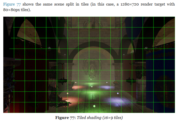
-
-
-
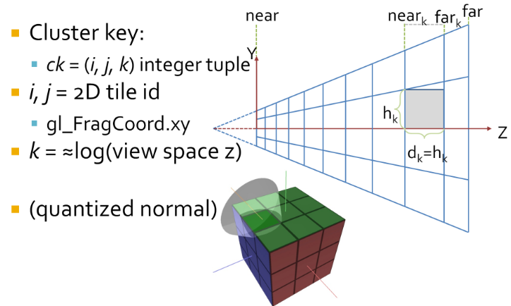 .
.
-
Cluster assignments is a simple mapping from sample coordinate, to an integer tuple
i,j,k. -
iandjare the tile coordinates, which can be derived by dividinggl_FragCoord.xyby the tile size.-
i = bx_screen_space/txcj = by_screen_space/tyc.
-
-
kis a logarithmic function of the view space Z of the sample, not simply the logarithm.-
The logarithmic subdivisions also means that as clusters become larger further away, we get a kind of LOD behaviour and do not end up with insane numbers of clusters, for a wide range of view parameters.
-
-
We use this subdivision as it creates self similar clusters that are as cube like as possible. This makes them better suited for culling.
-
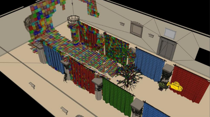 .
.
-
An easy solution is to use Axis Aligned Bounding Boxes (AABB) that enclose each cluster. AABBs built from the max and min points of the clusters will be ever so slightly larger than the actual clusters. We’re okay with this since it ensures that there are no gaps in between volumes due to precision issues. Also, AABB’s can be stored using only only two vec3’s, a max and min point.
-
This compute shader is ran once per cluster and aims to obtain the min and max points of the AABB encompassing said cluster.
-
First, imagine we’re looking at the view frustum from a front camera perspective, like we did in the Tiled Shading animations of part one. Each tile will have a min and max point, which in our coordinate system will be the upper right and bottom left vertices of a tile respectively. After obtaining these two points in screen space we set their Z position equal to the near plane, which in NDC and in my specific setup is equal to -1.
-
I know, I know. I should be using reverse Z, not the default OpenGL layout, I’ll fix that eventually.
-
-
Then, we transform these min and max points to view space. Next, we obtain the Z value of the “near” and “far” plane of our target mini-frustum / cluster. And, armed with the knowledge that all rays meet at the origin in view space, a pair of min and max values in screen space and both bounding planes of the cluster, we can obtain the four points intersecting those planes that will represent the four corners of the AABB encompassing said cluster. Lastly, we find the min and max of those points and save their values to the cluster array. And voilà, the grid is complete!
-
Screen To View:
-
Converts a given point in screen space to view space by taking the reverse transformation steps taken by the graphics pipeline.
-
-
Line Intersection to Z Plane:
-
Used to obtain the points on the corners of the AABB that encompasses a cluster. The normal vector of the planes is fixed at 1.0 in the z direction because we are evaluating the points in view space and positive z points towards the camera from this frame of reference.
-
-
When to recalculate:
-
Our list of cluster AABBs will be valid as long as the view frustum stays the same shape. So, it can be calculated once at load time and only recalculated with any changes in FOV or other view field altering camera properties.
-
My initial profiling in RenderDoc seems to indicate that the GPU can run this shader really quickly, so I think it wouldn’t be a huge deal either if this was done every frame.
-
Idk
-
From depth to froxel :
-
Given a near plane $n$, a far plane $m$, a maximum number of depth slices $z$ and a linear depth value in the range
[0..1], this equation can be used to compute the index of the cluster for a given position. -
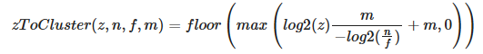 .
.
-
This formula suffers however from the resolution issue mentioned previously. We can fix it by introducing $sn$, a special near value that defines the extent of the first froxel (the first froxel occupies the range
[n..sn], the remaining froxels[sn..f]). -
The following equation can be used to compute a linear depth value from
gl_FragCoord.z(assuming a standard OpenGL projection matrix). -
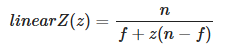 .
.
-
This equation can be simplified by pre-computing two terms $c0$ and $c1$:
-
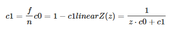 .
.
-
This simplification is important because we will pass the linear $z$ value to a
log2. Since the division becomes a negation under a logarithmic, we can avoid a division by using-log2(z * c0 + c1)instead. -
Implementation to compute a froxel index from a fragment's screen coordinates:
#define MAX_LIGHT_COUNT 16 // max number of lights per froxel uniform uvec4 froxels; // res x, res y, count y, count y uniform vec4 zParams; // c0, c1, index scale, index bias uint getDepthSlice() { return uint(max(0.0, log2(zParams.x * gl_FragCoord.z + zParams.y) * zParams.z + zParams.w)); } uint getFroxelOffset(uint depthSlice) { uvec2 froxelCoord = uvec2(gl_FragCoord.xy) / froxels.xy; froxelCoord.y = (froxels.w - 1u) - froxelCoord.y; uint index = froxelCoord.x + froxelCoord.y * froxels.z + depthSlice * froxels.z * froxels.w; return index * MAX_FROXEL_LIGHT_COUNT; } uint slice = getDepthSlice(); uint offset = getFroxelOffset(slice); // Compute lighting...-
Several uniforms must be pre-computed to perform the index evaluation efficiently.
froxels[0] = TILE_RESOLUTION_IN_PX; froxels[1] = TILE_RESOLUTION_IN_PX; froxels[2] = numberOfTilesInX; froxels[3] = numberOfTilesInY; zParams[0] = 1.0f - Z_FAR / Z_NEAR; zParams[1] = Z_FAR / Z_NEAR; zParams[2] = (MAX_DEPTH_SLICES - 1) / log2(Z_SPECIAL_NEAR / Z_FAR); zParams[3] = MAX_DEPTH_SLICES; -
-
From froxel to depth :
-
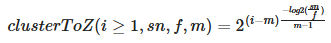 .
.
-
For $i = 0$, the z value is 0. The result of this equation is in the
[0..1]range and should be multiplied by $f$ to get a distance in world units. -
The compute shader implementation should use
exp2instead of apow. The division can be precomputed and passed as a uniform.
-
Data Structure
-
They’re implemented solely on the GPU using shader storage buffer objects, so keep in mind that reads and writes have incoherent memory access and will require the appropriate barriers to avoid any disasters.
-
 .
.
-
"At the end, you get an accelerated structure like this, which is just a grid where you can look up your light lists."
-
-
Global Light List :
-
It is an array containing all of the lights in a given scene with a size equivalent to the maximum amount of lights possible in the scene.
-
-
Global Light Index List :
-
Every light will have its own unique index based on its location in the Global Light List and that index is stored in the Global Light Index List.
-
This array contains the indices of all of the active lights in the scene grouped by cluster.
-
-
Light Grid :
-
Contain information as to how these indices relate to their parent clusters.
-
This array has as many elements as there are clusters and each element contains two unsigned ints, one that stores the offset to the Global Light Index List and another that contains the number of lights intersecting the cluster.
-
Each cell stores an offset and count that represent a range in ?.
-
This range contains a list of light indices indicating all the lights that the may affect the samples in the tile.
-
The Light Grid provides access to light list for each pixel.
-
-
Unlike what’s shown in the diagram, the global light index list does not necessarily store the indices for each cluster sequentially, in fact, it might store them in a completely random order.
-
If you’re wondering why we need such a convoluted data structure, the quick answer is that it plays nicely with the GPU and works well in parallel. Also, it allows both compute shaders and pixel shaders to read the same data structure and execute the same code. Lastly, it is pretty memory efficient since clusters tend to share the same lights and by storing indices to the global light list instead of the lights themselves we save up memory.
-
-
Check lights against every cluster of the view frustum. Performs light culling for every cluster in the cluster grid.
-
Thread groups sizes are actually relevant in this compute shader since I’m using shared GPU memory to reduce the number of reads and writes by only loading each light once per thread group, instead of once per cluster.
-
First, each thread gets its bearings and begins by calculating some initialization values.
-
For example, how many threads there are in a thread group, what it’s linear cluster index is and in how many passes it shall traverse the global light list.
-
-
Next, each thread initializes a count variable of how many lights intersect its cluster and a local index light array to zero.
-
Once setup is complete, each thread group begins a traversal of a batch of lights. Each individual thread will be responsible for loading a light and writing it to shared memory so other threads can read it.
-
A barrier after this step ensures all threads are done loading before continuing.
-
Then, each thread performs collision detection for its cluster, using the AABB we determined in step one, against every light in the shared memory array, writing all positive intersections to the local thread index array.
-
We repeat these steps until every light in the global light array has been evaluated.
-
Next, we atomically add the local number of active lights in a cluster to the globalIndexCount and store the global count value before we add to it.
-
This number is our offset to the global light index list and due to the nature of atomic operations we know that it will be unique per cluster , since only one thread has access to it at any given time.
-
Then, we populate the global light index list by transferring the values from the local light index list (named visibleLightIndices in the code) into the global light index list starting at the offset index we just obtained.
-
Finally, we write the offset value and the count of how many lights intersected the cluster to the lightGrid array at the given cluster index.
-
-
Once this shader is done running the data structures will contain all of the values necessary for a pixel shader to read the list of lights that are affecting a given fragment, since we can use the getClusterIndex function from the previous section to find which cluster a fragment belongs to.
-
With this, we’ve completed step five and therefore have all the building blocks in place for a working clustered shading implementation.
-
Even this simple culling method will still manage lights in the order of tens of thousands.
-
Extra Optimizations :
-
Jeremiah Van Oosten’s thesis writes about optimizing Clustered Renderers and has links to his testing framework where you can compare different efficient rendering algorithms.
-
He goes into detail as to how spatial optimization structures like Boundary Volume Hierarchies (BVH) and efficient light sorting can significantly increase performance and allow for scenes with millions of dynamic light sources in real-time.
-
Right now, it seems that implementing the BVH will be my first task — and specially after how important being familiar with BVH’s will become after Turing.
-
-
virtual shadow mapping enables hundreds of real-time shadow casting dynamic lights.
-
It should be considered an alternate clustering method best suited for mobile hardware.
-
Doom 2016 goes into optimized shaders to make use of GCN scalar units and saved some Vector General-Purpose Registers(VGPR). Also, by voxelizing environment probes, decals and lights the benefits of the cluster data structure were brought over to nearly all items that influence lighting.
-
-
Avalanche Studios :
-
Given a screen position and a depth value (whether from a depth buffer or the rasterized depth in a forward pass) we start by looking up the cluster from a 3D texture. Each texel represents a cluster and its light list.
-
The red channel gives us an offset to where the light list starts, whereas the green channel contains the light counts. The light lists are then stored in a tightly packed lists of indexes to the lights. The actual light source data is stored as arrays in a constant buffer.
-
All in all the data structure is very compact. In a typical artists lit scene it may be around 50- 100kb of data to upload to the GPU every frame.
-
 .
.
-
Data coherency :
-
So the difference between tiled and clustered is that we pick a light list on a per-pixel basis instead of per-tile, depending on which cluster we fall within. Obviously though, in a lot of cases nearby pixels will choose the same light list, in particular neighbors within the same tile on a similar depth. If we visualize what light lists were chosen, we can see that there are a bunch of different paths taken beyond just the tile boundaries. A number of depth discontinuities from the foliage in front of the player gets clearly visible. This may seem like a big problem, but here we are only talking about fetching different data. This is not a problem for a GPU, it’s something they do all the time for regular texture fetches, and this is even much lower frequency than that.
-
-
-
Filament Engine :
-
The list of lights per froxel can be passed to the fragment shader either as an SSBO or a texture.
-
During the rendering pass, we can compute the ID of the froxel a fragment belongs to and therefore the list of lights that can affect that fragment.
-
Finding Active Clusters / Unique Clusters
-
Motivation :
-
This section is optional since active cluster determination is not a crucial part of light culling.
-
Even though it isn’t terribly optimal, you can simply perform culling checks for all clusters in the cluster grid every frame.
-
Thankfully, determining active clusters doesn’t take much work to implement and can speed up the light culling pass considerably.
-
The only drawback is that it will require a Depth Pre-pass .
-
-
Depth Pre-pass :
-
The depth map generated is used to determine the minimum and maximum depth values within a tile, that is the minimum and maximum depths across the entire tile.
-
-
The key idea is that not all clusters will be visible all of the time, and there is no point in performing light culling against clusters you cannot see.
-
So, we can check every pixel in parallel for their cluster ID and mark it as active on a list of clusters.
-
This list will most likely be sparsely populated, so we will compact it into another list using atomic operations.
-
Then, during light culling we will check light “collisions” against the compacted list instead, saving us from having to check every light for every cluster.
-
To increase efficiency, both Van Oosten and Olsson compact this list into a set of unique clusters .
-
We compact the grid into the list of non-zero elements.
-
This leaves us with a list of clusters which needs lights assigned to them.
-
The most obvious method to find the unique clusters in parallel is to simply sort the cluster keys, and then perform a compaction step that removes any with an identical neighbour .
-
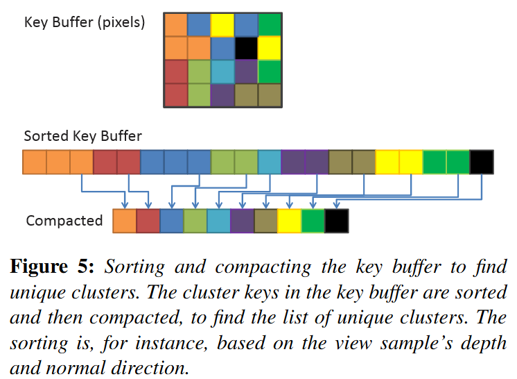 .
.
-
-
Identifying unique clusters :
-
Local Sorting
-
We sort samples in each screen space tile locally. This allows us to perform the sorting operation in on-chip shared memory, and use local (and therefore smaller) indices to link back to the source pixel.
-
We extract unique clusters from each tile using a parallel compaction. From this, we get the globally unique list of clusters. During the compaction, we also compute and store a link from each sample to its associated cluster.
-
-
Page Tables-
The second technique is similar to the page table approach used by virtual textures (Section 2). However, as the range of possible cluster keys is very large, we cannot use a direct mapping between cluster key and physical storage location for the cluster data; it simply would typically not fit into GPU memory. Instead we use a virtual mapping, and allocate physical pages where any actual keys needs storage. Lefohn et.al. [LSK∗06] provide details on software GPU implementation of virtual address translation. We exploit the fact that all physical pages are allocated in a compact range, and we can therefore compact that range to find the unique clusters.
-
-
Other methods:-
Both sorting and compaction are relatively efficient and readily available GPU building blocks. However, despite steady progress, sorting remains an expensive operation.
-
Methods that rely on adjacent screen-space coherency are not robust, especially with respect to stochastic frame buffers.
-
We therefore focus on techniques that do not suffer from this weaknesses.
-
-
-
Explicit Bounds :
-
As the actual view-sample positions and normals typically have tighter bounds, we also evaluate explicit 3D bounds and normal cones.
-
We compute the explicit bounds by performing a reduction over the samples in each cluster (e.g., we perform a min-max reduction to find the AABB enclosing each cluster).
-
The results of the reduction are stored separately in memory.
-
When using page tables, the reduction is difficult to implement efficiently, because of the many-to-one mapping from view samples to cluster data, we would need to make use of atomic operations, and get a high rate of collisions. We deemed this to be impractically expensive.
-
We therefore only implement explicit bounds for local sort.
-
After the local sort, information about which samples belong to a given cluster is readily available.
-
-
//Input
vec2 pixelID; // The thread x and y id corresponding to the pixel it is representing
vec2 screenDimensions; // The total pixel size of the screen in x and y

//Output
bool clusterActive[];

//We will evaluate the whole screen in one compute shader
//so each thread is equivalent to a pixel
void markActiveClusters(){
    //Getting the depth value
    vec2 screenCord = pixelID.xy / screenDimensions.xy;
    float z = texture(screenCord) //reading the depth buffer

    //Getting the linear cluster index value
    uint clusterID = getClusterIndex(vec3(pixelID.xy, z));
    clusterActive[clusterID] = true;
}
//Input
vec3 pixelCoord;  // Screen space pixel coordinate with depth
uint tileSizeInPx; // How many pixels a rectangular cluster takes in x and y
uint3 numClusters; // The fixed number of clusters in x y and z axes

//Output
uint clusterIndex; // The linear index of the cluster the pixel belongs to

uint getClusterIndex(vec3 pixelCoord){
    // Uses equation (3) from Building a Cluster Grid section
    uint clusterZVal  = getDepthSlice(pixelCoord.z);

    uvec3 clusters    = uvec3( uvec2( pixelCoord.xy / tileSizeInPx), clusterZVal);
    uint clusterIndex = clusters.x +
                        numClusters.x * clusters.y +
                        (numClusters.x * numClusters.y) * clusters.z;
    return clusterIndex;
}
//Input
bool clusterActive[]; //non-compacted list
uint globalActiveClusterCount; //Number of active clusters

//Output
uint uniqueActiveClusters[]; //compacted list of active clusters

//One compute shader for all clusters, one cluster per thread
void buildCompactClusterList(){
    uint clusterIndex  = gl_GlobalInvocationID;
    if(clusterActive[clusterIndex]){
       uint offset = atomicAdd(globalActiveClusterCount, 1);
       uniqueActiveClusters[offset] = clusterIndex;
    }
}
Light Culling / Light Assignment
-
This step aims to assign lights to each cluster based on their view space position.
-
The main idea is that we perform something very similar to a “light volume collision detection” against the active clusters in the scene and append any lights within a cluster to a local list of lights.
-
Performing this “light volume collision detection” requires that I define clearly what I mean by light volume .
-
In a nutshell, lights become dimmer with distance. After a certain point they are so dim we can assume they aren’t contributing to shading anymore so, we mark those points as our boundary. The volume contained within the boundary is our light volume and if that volume intersects with the AABB of a cluster, we assume that light is contained within the cluster.
//Input:
uint light; // A given light index in the shared lights array
uint tile;  // The cluster index we are testing

//Checking for intersection given a cluster AABB and a light volume
bool testSphereAABB(uint light, uint tile){
    float radius = sharedLights[light].range;
    vec3 center  = vec3(viewMatrix * sharedLights[light].position);
    float squaredDistance = sqDistPointAABB(center, tile);

    return squaredDistance <= (radius * radius);
}
-
The main idea is that we check the distance between the point light sphere center and the AABB. If the distance is less than the radius they are intersecting.
-
For spotlights, the light volume and consequently the collision tests will be very different.
-
Check out this presentation by Emil Persson that explains how they implemented spotlight culling in Just Cause 3 if you do want to know more.
-
Light Assignment
-
The lights have a limited range, with some falloff which goes to 0 at the boundary.
-
There is no pre-computation so all geometry and lights are allowed to change freely from frame to frame.
-
The goal of the light assignment stage is to calculate the list of lights influencing each cluster. Previous designs for tiled deferred shading implementations have by and large utilized a brute force approach to finding the intersection between lights and tiles. That is, light-cluster overlaps were found by, for each tile, iterating over all lights in the scene and testing bounding volumes. This is tolerable for reasonably low numbers of lights and clusters.
-
To support large numbers of lights and a dynamically varying number of clusters, we use a fully hierarchical approach based on a spatial tree over the lights.
-
Each frame, we construct a bounding volume hierarchy (BVH) by first sorting the lights according to the Z-order (Morton Code) based on the discretized centre position of each light. We derive the discretization from a dynamically computed bounding volume around all lights.
-
We use a BVH with a branching factor of 32, which is rebuilt each frame.
-
When not so many lights are used, there are many other approaches which may be better.
-
-
The leaves of the search tree we get directly from the sorted data.
-
Next, 32 consecutive leaves are grouped into a bounding volume (AABB) to form the first level above the leaves.
-
The next level is constructed by again combining 32 consecutive elements. We continue until a single root element remains.
-
For each cluster, we traverse this BVH using depth-first traversal. At each level, the bounding box of the cluster (either explicitly computed from the cluster’s contents or implicitly derived from the cluster’s key) is tested against the bounding volumes of the child nodes. For the leaf nodes, the sphere bounding the light source is used; other nodes store an AABB enclosing the node. The branching factor of 32 allows efficient SIMD-traversal on the GPU and keeps the search tree relatively shallow (up to 5 levels), which is used to avoid expensive recursion (the branching factor should be adjusted depending on the GPU used, the factor of 32 is convenient on current NVIDIA GPUs).
-
If a normal cone is available for a cluster, we use this cone to further reject lights that will not affect any samples in the cluster; etc (to summarize).
-
Avalanche Studios :
-
Deriving the explicit cluster bounds was something that could be interesting, but we found that sticking to implicit bounds simplified the technique, while also allowing the light assignment to run on the CPU.
-
In addition, this gives us scene independence. This means that we don’t need to know what the scene looks like to fill in the clusters, and this also allows us to evaluate light at any given point in space, even if it’s floating in thin air. This could be relevant for instance for ray-marching effects.
-
Given that we are doing the light assignment on the CPU, one may suspect that this will become a significant burden for the CPU. However, our implementation is fast enough to actually save us a bunch of CPU time over our previous solution. In a normal artist lit scene we recorded 0.1ms on one core for clustered shading. The old code supporting our previous forward pass for transparency that was still running in our system was still consuming 0.67ms for the same scene, a cost that we can now eliminate.
-
-
Filament Engine :
-
Before rendering a frame, each light in the scene is assigned to any froxel it intersects with. The result of the lights assignment pass is a list of lights for each froxel.
-
Lights assignment can be done in two different ways, on the GPU or on the CPU.
-
On GPU:
-
The lights are stored in Shader Storage Buffer Objects (SSBO) and passed to a compute shader that assigns each light to the corresponding froxels.
-
The lights assignment can be performed each frame by another compute shader.
-
The threading model of compute shaders is particularly well suited for this task. We simply invoke as many workgroups as we have froxels (we can directly map the X, Y and Z workgroup counts to our froxel grid resolution). Each workgroup will in turn be threaded and traverse all the lights to assign.
-
Intersection tests imply simple sphere/frustum or cone/frustum tests.
-
Assigning Lights with Froxels :
-
Assigning lights to froxels can be implemented on the GPU using two compute shaders.
-
The first one, creates the froxels data (4 planes + a min Z and max Z per froxel) in an SSBO and needs to be run only once.
-
Projection matrix
-
The projection matrix used to render the scene (view space to clip space transformation).
-
-
Inverse projection matrix
-
The inverse of the projection matrix used to render the scene (clip space to view space transformation).
-
-
Depth parameters
-
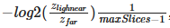 , maximum number of depth slices, Z near and Z far.
-
-
Clip space size
-
 , with $F_x$ the number of tiles on the X axis, $F_r$ the resolution in pixels of a tile and w the width in pixels of the render target.
-
-
#version 310 es precision highp float; precision highp int; #define FROXEL_RESOLUTION 80u layout(local_size_x = 1, local_size_y = 1, local_size_z = 1) in; layout(location = 0) uniform mat4 projectionMatrix; layout(location = 1) uniform mat4 projectionInverseMatrix; layout(location = 2) uniform vec4 depthParams; // index scale, index bias, near, far layout(location = 3) uniform float clipSpaceSize; struct Froxel { // NOTE: the planes should be stored in vec4[4] but the // Adreno shader compiler has a bug that causes the data // to not be read properly inside the loop vec4 plane0; vec4 plane1; vec4 plane2; vec4 plane3; vec2 minMaxZ; }; layout(binding = 0, std140) writeonly restrict buffer FroxelBuffer { Froxel data[]; } froxels; shared vec4 corners[4]; shared vec2 minMaxZ; vec4 projectionToView(vec4 p) { p = projectionInverseMatrix * p; return p / p.w; } vec4 createPlane(vec4 b, vec4 c) { // standard plane equation, with a at (0, 0, 0) return vec4(normalize(cross(c.xyz, b.xyz)), 1.0); } void main() { uint index = gl_WorkGroupID.x + gl_WorkGroupID.y * gl_NumWorkGroups.x + gl_WorkGroupID.z * gl_NumWorkGroups.x * gl_NumWorkGroups.y; if (gl_LocalInvocationIndex == 0u) { // first tile the screen and build the frustum for the current tile vec2 renderTargetSize = vec2(FROXEL_RESOLUTION * gl_NumWorkGroups.xy); vec2 frustumMin = vec2(FROXEL_RESOLUTION * gl_WorkGroupID.xy); vec2 frustumMax = vec2(FROXEL_RESOLUTION * (gl_WorkGroupID.xy + 1u)); corners[0] = vec4( frustumMin.x / renderTargetSize.x * clipSpaceSize - 1.0, (renderTargetSize.y - frustumMin.y) / renderTargetSize.y * clipSpaceSize - 1.0, 1.0, 1.0 ); corners[1] = vec4( frustumMax.x / renderTargetSize.x * clipSpaceSize - 1.0, (renderTargetSize.y - frustumMin.y) / renderTargetSize.y * clipSpaceSize - 1.0, 1.0, 1.0 ); corners[2] = vec4( frustumMax.x / renderTargetSize.x * clipSpaceSize - 1.0, (renderTargetSize.y - frustumMax.y) / renderTargetSize.y * clipSpaceSize - 1.0, 1.0, 1.0 ); corners[3] = vec4( frustumMin.x / renderTargetSize.x * clipSpaceSize - 1.0, (renderTargetSize.y - frustumMax.y) / renderTargetSize.y * clipSpaceSize - 1.0, 1.0, 1.0 ); uint froxelSlice = gl_WorkGroupID.z; minMaxZ = vec2(0.0, 0.0); if (froxelSlice > 0u) { minMaxZ.x = exp2((float(froxelSlice) - depthParams.y) * depthParams.x) * depthParams.w; } minMaxZ.y = exp2((float(froxelSlice + 1u) - depthParams.y) * depthParams.x) * depthParams.w; } if (gl_LocalInvocationIndex == 0u) { vec4 frustum[4]; frustum[0] = projectionToView(corners[0]); frustum[1] = projectionToView(corners[1]); frustum[2] = projectionToView(corners[2]); frustum[3] = projectionToView(corners[3]); froxels.data[index].plane0 = createPlane(frustum[0], frustum[1]); froxels.data[index].plane1 = createPlane(frustum[1], frustum[2]); froxels.data[index].plane2 = createPlane(frustum[2], frustum[3]); froxels.data[index].plane3 = createPlane(frustum[3], frustum[0]); froxels.data[index].minMaxZ = minMaxZ; } }-
The second compute shader, runs every frame (if the camera and/or lights have changed) and assigns all the lights to their respective froxels.
-
Light index buffer
-
For each froxel, the index of each light that affects said froxel. The indices for point lights are written first and if there is enough space left, the indices for spot lights are written as well. A sentinel of value 0×7fffffffu separates point and spot lights and/or marks the end of the froxel's list of lights. Each froxel has a maximum number of lights (point + spot).
-
-
Point lights buffer
-
Array of structures describing the scene's point lights.
-
-
Spot lights buffer
-
Array of structures describing the scene's spot lights.
-
-
Froxels buffer
-
The list of froxels represented by planes, created by the previous compute shader.
-
-
#version 310 es precision highp float; precision highp int; #define LIGHT_BUFFER_SENTINEL 0x7fffffffu #define MAX_FROXEL_LIGHT_COUNT 32u #define THREADS_PER_FROXEL_X 8u #define THREADS_PER_FROXEL_Y 8u #define THREADS_PER_FROXEL_Z 1u #define THREADS_PER_FROXEL (THREADS_PER_FROXEL_X * \ THREADS_PER_FROXEL_Y * THREADS_PER_FROXEL_Z) layout(local_size_x = THREADS_PER_FROXEL_X, local_size_y = THREADS_PER_FROXEL_Y, local_size_z = THREADS_PER_FROXEL_Z) in; // x = point lights, y = spot lights layout(location = 0) uniform uvec2 totalLightCount; layout(location = 1) uniform mat4 viewMatrix; layout(binding = 0, packed) writeonly restrict buffer LightIndexBuffer { uint index[]; } lightIndexBuffer; struct PointLight { vec4 positionFalloff; // x, y, z, falloff vec4 colorIntensity; // r, g, b, intensity vec4 directionIES; // dir x, dir y, dir z, IES profile index }; layout(binding = 1, std140) readonly restrict buffer PointLightBuffer { PointLight lights[]; } pointLights; struct SpotLight { vec4 positionFalloff; // x, y, z, falloff vec4 colorIntensity; // r, g, b, intensity vec4 directionIES; // dir x, dir y, dir z, IES profile index vec4 angle; // angle scale, angle offset, unused, unused }; layout(binding = 2, std140) readonly restrict buffer SpotLightBuffer { SpotLight lights[]; } spotLights; struct Froxel { // NOTE: the planes should be stored in vec4[4] but the // Adreno shader compiler has a bug that causes the data // to not be read properly inside the loop vec4 plane0; vec4 plane1; vec4 plane2; vec4 plane3; vec2 minMaxZ; }; layout(binding = 3, std140) readonly restrict buffer FroxelBuffer { Froxel data[]; } froxels; shared uint groupLightCounter; shared uint groupLightIndexBuffer[MAX_FROXEL_LIGHT_COUNT]; float signedDistanceFromPlane(vec4 p, vec4 plane) { // plane.w == 0.0, simplify computation return dot(plane.xyz, p.xyz); } void synchronize() { memoryBarrierShared(); barrier(); } void main() { if (gl_LocalInvocationIndex == 0u) { groupLightCounter = 0u; } memoryBarrierShared(); uint froxelIndex = gl_WorkGroupID.x + gl_WorkGroupID.y * gl_NumWorkGroups.x + gl_WorkGroupID.z * gl_NumWorkGroups.x * gl_NumWorkGroups.y; Froxel current = froxels.data[froxelIndex]; uint offset = gl_LocalInvocationID.x + gl_LocalInvocationID.y * THREADS_PER_FROXEL_X; for (uint i = 0u; i < totalLightCount.x && groupLightCounter < MAX_FROXEL_LIGHT_COUNT && offset + i < totalLightCount.x; i += THREADS_PER_FROXEL) { uint currentLight = offset + i; vec4 center = pointLights.lights[currentLight].positionFalloff; center.xyz = (viewMatrix * vec4(center.xyz, 1.0)).xyz; float r = inversesqrt(center.w); if (-center.z + r > current.minMaxZ.x && -center.z - r <= current.minMaxZ.y) { if (signedDistanceFromPlane(center, current.plane0) < r && signedDistanceFromPlane(center, current.plane1) < r && signedDistanceFromPlane(center, current.plane2) < r && signedDistanceFromPlane(center, current.plane3) < r) { uint index = atomicAdd(groupLightCounter, 1u); groupLightIndexBuffer[index] = currentLight; } } } synchronize(); uint pointLightCount = groupLightCounter; offset = froxelIndex * MAX_FROXEL_LIGHT_COUNT; for (uint i = gl_LocalInvocationIndex; i < pointLightCount; i += THREADS_PER_FROXEL) { lightIndexBuffer.index[offset + i] = groupLightIndexBuffer[i]; } if (gl_LocalInvocationIndex == 0u) { if (pointLightCount < MAX_FROXEL_LIGHT_COUNT) { lightIndexBuffer.index[offset + pointLightCount] = LIGHT_BUFFER_SENTINEL; } } } -
-
-
On CPU:
-
The algorithm is different from the GPU implementation. Instead of iterating over every light for each froxel, the engine will “rasterize” each light as froxels. For instance, given a point light’s center and radius, it is trivial to compute the list of froxels it intersects with.
-
This technique has the added benefit of providing tighter culling than in the GPU variant. The CPU implementation can also more easily generate a packed list of lights.
-
-
Culling
-
Avalanche Studios :
-
Point light :
-
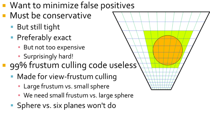 .
.
-
Our light sources are typically artist placed, scaled for human environments in an outdoor world, so generally speaking from meters to tens of meters. So a light source generally intersects many clusters. The typical sphere-frustum tests that you can find online are not suitable for this sort of culling. They are made for view-frustum culling and based on the assumption that the frustum typically is much larger than the sphere, which is the opposite of what we have here. Typically they simply test sphere vs plane for each six planes of the frustum. This is conservative, but lets through spheres that aren’t completely behind any of the planes, such as in the frustum corners. The result you get is that green rectangle, or essentially a ”cube” of clusters around the light. But that’s also the first thing we compute. We simply compute the screen-space and depth extents of the light analytically first, so this test doesn’t actually help anything at all after that.
-
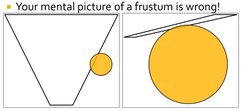 .
.
-
Most frustum culling code is written with the scenario on the left in mind. We need to handle the scenario on the right.
-
One way to go about frustum culling is testing all planes, all edges and all vertices. This would work, but be too costly to outweigh the gains from fewer false positives. A fast, conservative but relatively tight solution is what we are looking for. There are many approaches that seem fitting, but there are also many complications, which has ultimately thrown many of our attempts into the garbage bin. One relatively straightforward approach is to cull against the cluster’s AABB. This is fast and gives fairly decent results, but it’s possible to do better.
-
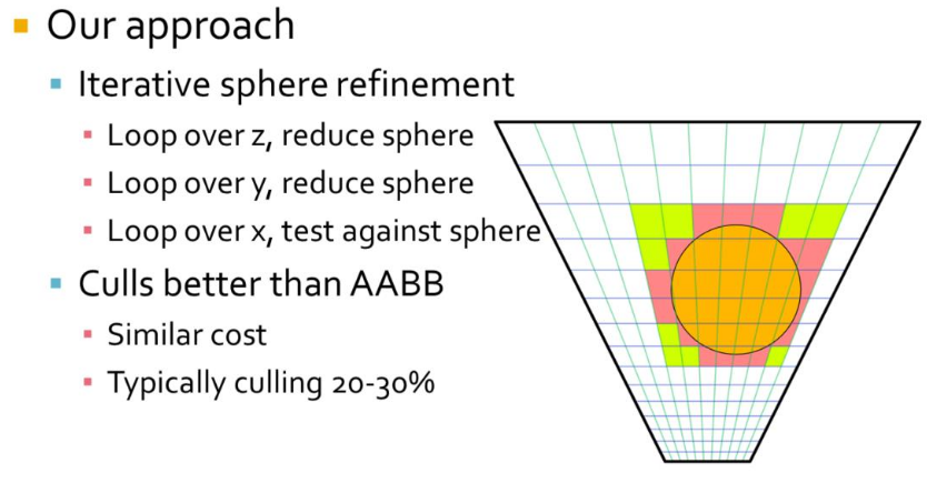
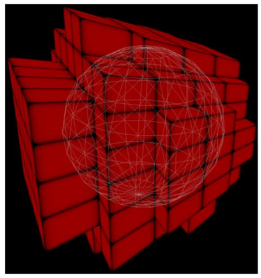 .
.
-
Starting with the ”cube” of clusters around the light, in our outer loop we iterate over the slices in z direction. We intersect the sphere with the slice where it is the widest. This results in a circle of a smaller radius than the original sphere, we thus continue in the y direction using a sphere of this smaller radius and the circle’s midpoint. In the center slice we simply proceed with the original sphere. We repeat this procedure in y and have an even smaller sphere. Then in the inner loop we do plane vs. sphere tests in x direction to get a strip of clusters to add the light to.
-
To optimize all the math we take advantage of the fact that in view-space, all planes will have components that are zero. A plane in the x direction will have zero y and offset, y direction has zero x and offset, and z-direction is basically only a z offset.
-
The resulting culling is somewhat tighter than a plain AABB test, and costs about the same. Where AABB culls around 15-25%, this technique culls around 20-30% from the “cube” of clusters.
-
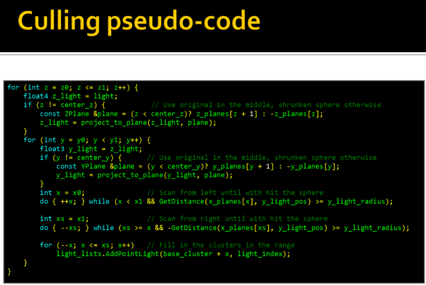 .
.
-
-
Spotlight :
-
For spotlights we begin by finding the ”cube” of clusters around the light’s sphere, just like for pointlights, except this cube typically is much larger than necessary for a spotlight. However, this analytical test is cheap and goes a long way to limit the search space for following passes. Next we find a tighter ”cube” simply by scanning in all six directions, narrowing it down by doing plane-cone tests. There is likely a neat analytical solution here, but this seemed non- trivial. Given that the plane scanning works fine and is cheap we haven’t really explored that path.
-
Note that our cones are sphere-capped rather than flat-capped. That’s because the light attenuation is based on distance (as it should), rather than depth. Sphere-capped cones also generally behave much better for wide angles and doesn’t become extremely large as flat-capped cones can get.
-
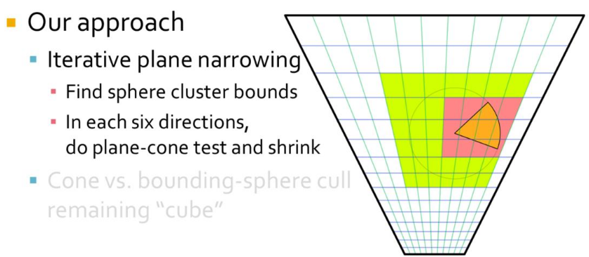
 .
.
-
Finally, for the remaining ”cube” of clusters we cull each cluster with a sphere-capped cone vs. bounding sphere test. For this to work well we have to have relatively cubical shaped clusters, otherwise the bounding sphere becomes way oversized. Overall this technique results in a moderately tight culling that is good enough for us so far, although there is room for some minor improvement.
-
-
Shading
-
Shading differs from Tiled Shading only in how we look up the cluster for the view sample in question.
-
For Tiled Shading, a simple 2D lookup, based on the screen-space coordinates, is sufficient to retrieve light-list offset and count. However, for clustered approaches, there no longer exists a direct mapping between the cluster key and the index into the list of unique clusters.
-
In the sorting approach, we explicitly store this index for each pixel. This is achieved by tracking references back to the originating pixel, and, when the unique cluster list is established, storing the index to the correct pixel in a full screen buffer.
-
When using page tables, after the unique clusters are found, we store the cluster index back to the physical memory location used to store the cluster key earlier (using the same page table as before). This means that a virtual lookup for the cluster key will yield the cluster index. Thus, each sample can look up the cluster index using the cluster key computed earlier (or re-computed).
Cluster Key Packing
-
For maximum performance when using sorting or page tables, we wish to pack the cluster key into as few bits as possible. We allocate 8 bits to each i and j components, which identify the screen-space tile the cluster belongs to. This allows up to 8192 × 8192 size render targets (assuming screen-space tile size of 32 × 32 pixels). The depth index k is determined from settings for the near and far planes and Equation 2. In our scenes, we found 10 bits to be sufficient. This leaves up to 6 bits for the optional normal clustering. Using 6 bits, we can for instance support a resolution up to 3 × 3 subdivisions on each cube face (3 × 3 × 6 = 54 and dlog2 54e = 6). For more restricted environments, the data could be packed more aggressively, saving both time and space.
Tile sorting
-
To the cluster key (between 10 and 16 bits wide) we attach an additional 10 bits of meta-data, which identifies the sample’s original position relative to its tile. We then perform a tile-local sort of the cluster keys and the associated meta-data. The sort only considers the up-to 16 bits of the cluster key; the meta-data is used as a link back to the original sample after sorting. In each tile, we count the number of unique cluster keys. Using a prefix operation over the counts from each tile, we find the total number of unique cluster keys and assign each cluster a unique ID in the range
[0...numClusters). We write the unique ID back to each pixel that is a member of the cluster. The unique ID also serves as an offset in memory to where the cluster’s data is stored. -
Bounding volumes (AABB and normal cone) can be re-constructed from the cluster keys, in which case each cluster only needs to store its cluster key. For explicit bounding volumes, we additionally store the AABB and/or normal cone. The explicit bounding volumes are computed using a reduction operation: for instance, AABBs can be found using a min- and a max-reduction operation on the sample positions. The meta-data from the locally sorted cluster keys gives us information on which samples belong to a given cluster.
Shadows
-
Efficient Virtual Shadow Maps for Many Lights - Ola Olsson - 2014 .
-
This paper builds on clustered shading.
-
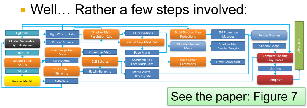 .
.
-
-
Etc :
-
I saw this in some paper and left it loose; maybe I’ll revisit it later.
-
Resolution Matched Shadow Maps (RMSM), must determine which shadow pages are used by the view samples. The method achieves this by first exploiting screen space coherency to reduce duplicate requests from adjacent pixels in screen space. Globally unique requests are then determined by sorting and compacting the remaining requests.
-
Garanzha present a similar technique that they call Compress-Sort-Decompress (CSD). Their goal is to find 3D (or 5D) clusters in a frame buffer, which are used to form ray packets. The main differences are that Garanzha et al. treat the frame buffer as a 1D sequence and use run length encoding (RLE) to reduce duplicates before sorting. They expand the result after the sorting.
-
The approaches in both RMSMs and CSD rely on the presence of coherency between adjacent input elements, in 2D and 1D respectively. In many cases, this is a reasonable assumption. However, techniques such as multi sampling anti aliasing (MSAA) with alpha-to-coverage, or stochastic transparency, invalidate this assumption. Coherency is still present in the frame buffer, but not between adjacent samples. For scenes with low coherence between adjacent samples, both of these methods degenerate to sorting the entire frame buffer.
-
-
It has even been stated that shadow maps are unsuited for many lights. However, when limiting the problem as I have just done, there really is no fundamental reason against shadow maps. And given that they are the de facto standard in the real-time industry, they must clearly be the first stop, if nothing else to provide a benchmark for more clever ideas.
-
To create shadow maps, we need to perform the following steps each frame, using the current camera view:
-
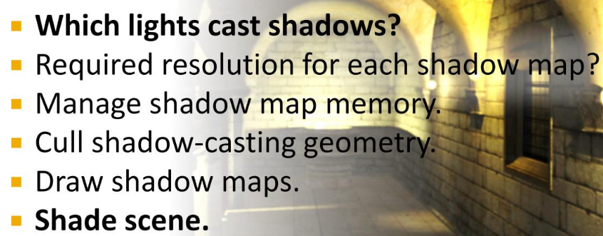 .
.
-
The first step is the same as determining what lights are needed for shading, and we have already seen how this can be achieved using clustered shading and other methods.
-
The last step is also fairly trivial, using bindless textures , array textures or shadow map atlases .
-
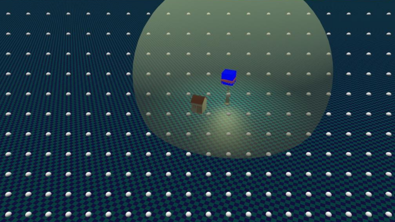
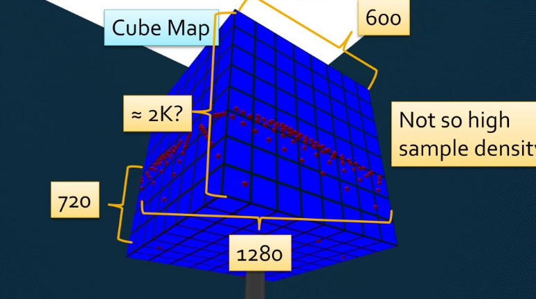 .
.
-
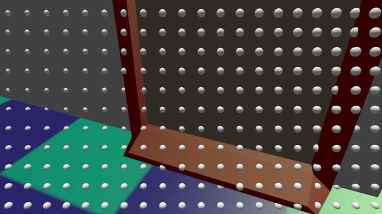
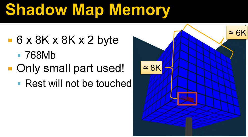 .
.
-
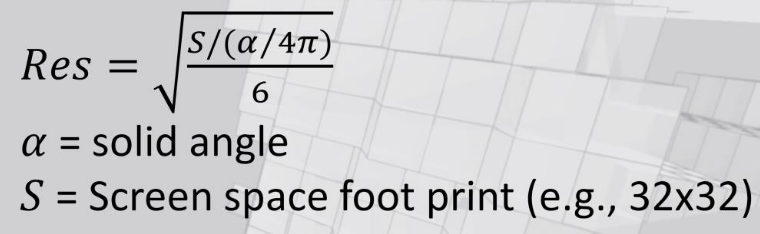 .
.
-
As we saw before, the shadow map samples can be very tightly grouped, requiring a high shadow map resolution And note how this happens when most of the shadow map would be unused! This is pretty much how it has to be, as the high density comes from looking at something very near the camera, and then we’re guaranteed to not see so very much of the scene. This is highly wasteful and a fantastic opportunity, for...
-
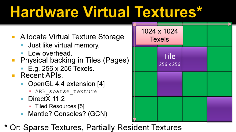 .
.
-
Keyword: Virtual Shadow Maps (Virtual SMs).
-
See pages 181 to 195 of Efficient Real-Time Shading with Many Lights - Ola Olsson, Emil Persson (Avalanche) - 2014 for more information.
-
-
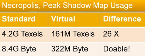 .
.
-
In other terms, this means the difference between impossible on a current console and something we might consider.
-
Our method achieves quite uniform shadow quality, this means we can control quality and thus memory usage with a global parameter. This allows more flexibility in memory use while maintaining uniform quality. An interesting idea is to do this dynamically, to ensure a certain memory budget. Should be possible as it is very quick to work out memory usage from the used pages and resolutions.
-
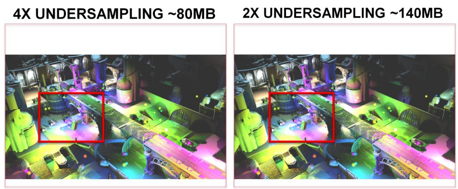
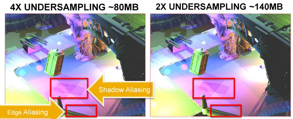 .
.
-
Recall that the peak is 322MB without reducing quality.
-
Cull Shadow Cast Geometry :
-
This process is just like normal view frustum culling, in that we are trying to get rid of geometry that is not visible, and that we do this by testing bounding volumes of chunks or batches of triangles.
-
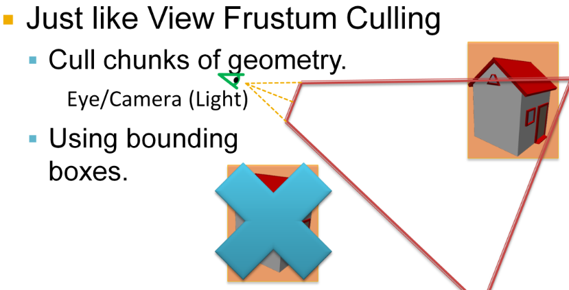
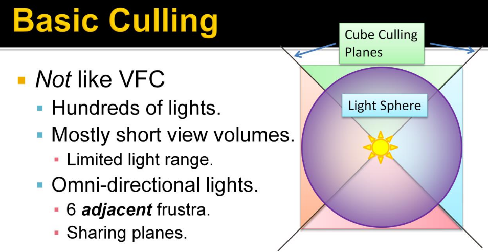 .
.
-
What is not like view frustum culling is that we need to perform hundreds of these tests. The view volumes are quite small, or short, given the limited range of the lights. There are 6 adjacent frustra sharing planes. This adjacency means we can share calculations.
-
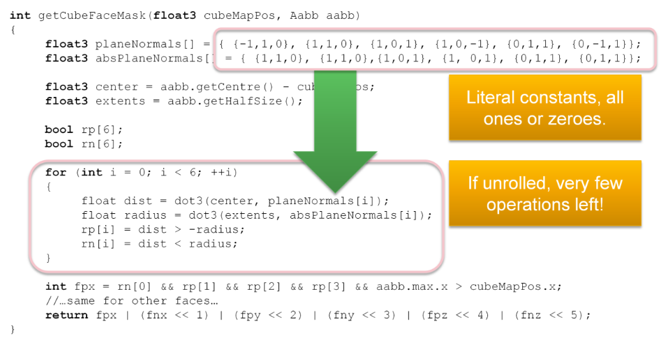 .
.
-
Here is the somewhat condensed code we use to calculate the culling mask, with a bit for each cube face. This is a very efficient test, checking only 6 planes for six frustums. Especially as the plane equations are all ones and zeroes, which means that if the loop is unrolled, most of this code just goes away. I think this is a rather big advantage with cube maps, over using separate frustums (As done in [6]). This efficiency is especially important given that we will be culling a lot more objects than normal culling!
-
You see, to enable efficient culling, batches must be small. Intuitively, for any culling, the optimal size of batches correlates to the size of the frustums. If batches are too large, the triangles get replicated into most cube faces.
-
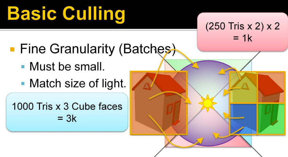 .
.
-
So we are trading increased culling work for fewer triangles drawn. Triangle drawing is the biggest performance bottleneck so this is important to be able to tune.
-
We used batches of up to 128 triangles, in practice they average around 68 triangles. A batch is represented by an AABB and a list of triangles. The batches are constructed in a pre-process, that builds a tree using agglomerative clustering (see the paper section 6.2.1). Note that the quality of the batches is fairly important for good performance. The batches are stored in a flat array that is loaded into the runtime.
-
These values remind me of "clusters in the rabbit". See Optimization Techniques -> Cluster.
-
-
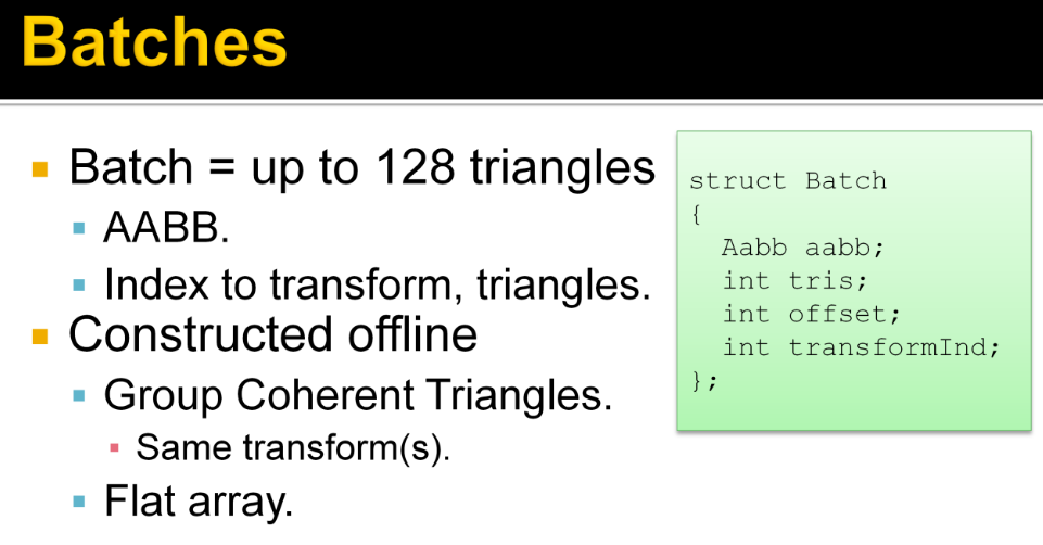 .
.
-
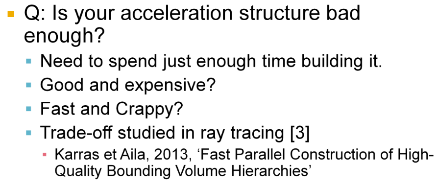 .
.
-
For efficient culling, we obviously need a hierarchy.
-
The important thing is to balance the time spent building and traversing an acceleration structure. This trade-off has been studied by Karras and Aila in context of ray tracing, and is a very interesting read. In short, it suggests to me that the acceleration structure for just a few thousand box queries must be pretty bad to be worth building.
-
We used a very simple, full, 32-way BVH which is completely rebuilt each frame. This is in no way the best possible structure, or even the fastest to build, but it has served us well.
-
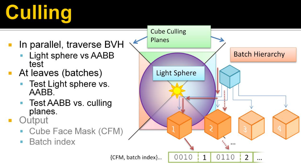 .
.
-
Here we parallelize the lights, and each light traverses the hierarchy to find the batches that overlap the sphere. These batches are those that may produce a shadow if drawn into the shadow map.
-
This produces a list for each light of pairs of cube face masks and batch indexes. The Cube Face Mask is a bit mask where each bit indicates if it overlaps a certain cube face. This tells us what batches to draw to which cube faces of each light.
-
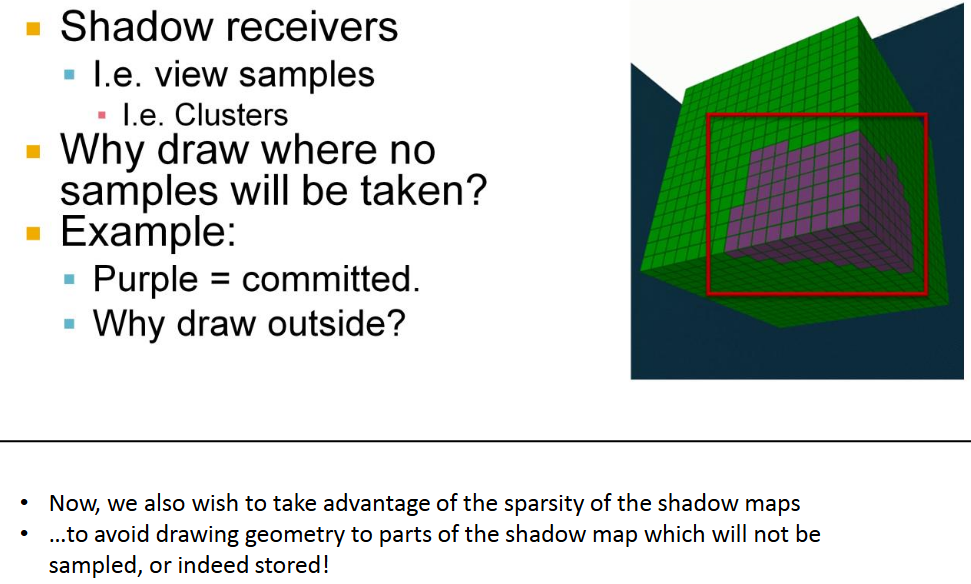 .
.
-
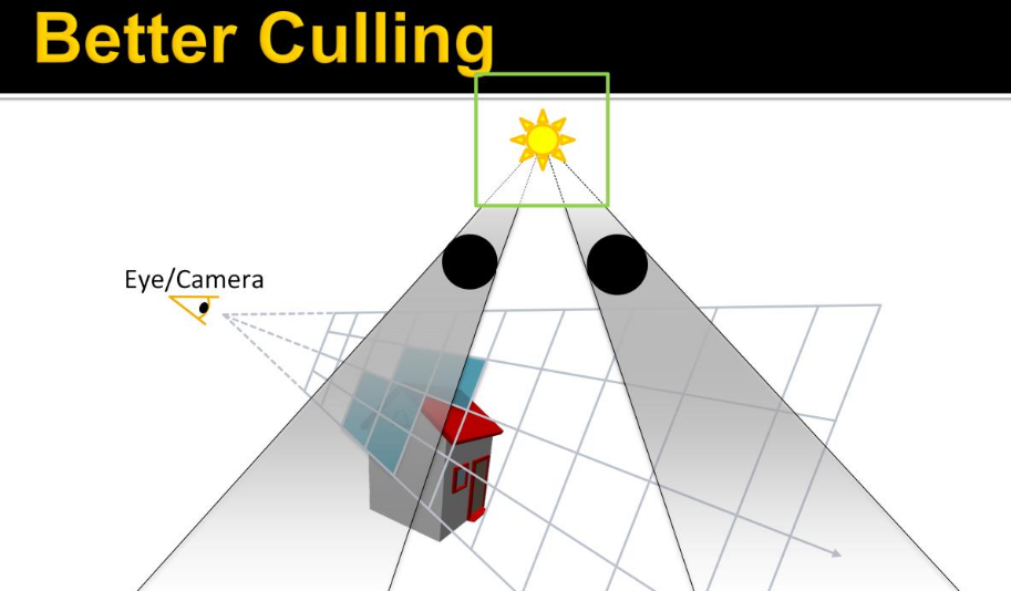 .
.
-
Green: source light BB.
-
Black: Shadow casters.
-
Blue: Clusters containing samples.
-
-
Note that the shadow casters are outside of the view volume, and so have no clusters associated, but cast their shadow through the view volume. So we’re interested in finding out what shadows affect the visible samples, and thus determine if the shadow caster needs to be drawn.
-
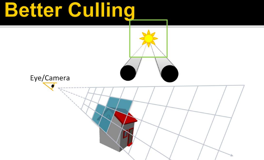 .
.
-
Instead of doing some crazy thing, like shadow volumes, we can figure this out by projecting the shadow caster onto the light source. This gives us these two intervals on the cube face.
-
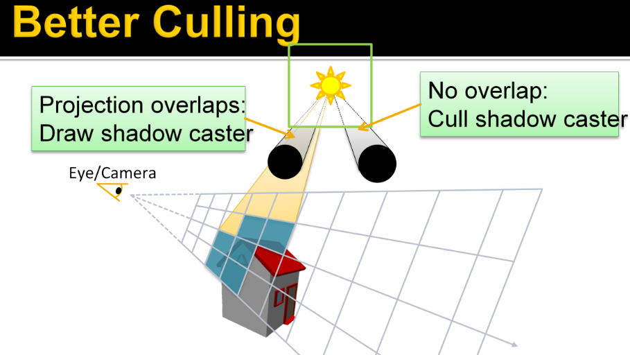 .
.
-
Doing the same thing for the clusters, gives us another interval. If the projection of a shadow caster overlaps that of some clusters, i.e. shadow receiver, …it needs to be rendered into this shadow map, else, it doesn’t. Note that the clusters don’t need to form a range for this to work, any overlap will do.
-
The subject continues from pages 225 to 243 of Efficient Real-Time Shading with Many Lights - Ola Olsson, Emil Persson (Avalanche) - 2014 .
-
I found it quite specific and complicated to implement, for something I'm not focusing on right now.
-
-
-
-
Avalanche Studios :
-
Classic deferred has the advantage that you can iterate light by light, and thus reuse resources such as shadow buffers in between. This saves some memory, which may be needed on current generation consoles. On PC and next-generation consoles this is not nearly as big a problem.
-
With the switch to clustered shading the cost of adding a new light to the scene is small. Artists can now be moderate ”wasteful” without causing much problems performance-wise. This is not true for rasterizing shadow buffers. They remain expensive, and relatively speaking going to be more expensive going forward since it’s often a ROP-bound process, and ROPs aren’t getting scaled up nearly as much as ALU. So we still need to be a bit conservative about how many shadow casting lights we add to the scene.
-
An observation that was made is that artists often place very similar looking lights close to each other. In some cases it is to get a desired profile of a light, in which case the two lights may in fact be centered at the exact same point. But often it is motivated by the real world, such as two headlights on car. Some vehicles actually have ten or more lights, all pointing in the same general direction. Rendering ten shadow buffers for that may prove to be far too expensive.
-
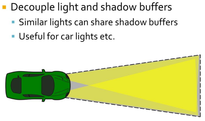 .
.
-
Often it works just fine to share a single shadow buffer for these lights. While the shadow may be slightly off, this is usually not something that you will notice unless you are specifically looking for it. To make this work the shadow buffer is decoupled from lights and the light is assigned a shadow buffer and frustum from which to extract shadows. The shadow frustum has to be large enough to include all the different lights that uses it.
-
Transparency
-
When the transparent geometry is considered, the depth range optimization cannot be fully used. Instead, only a more conventional hierarchical depth test can be used. The grid structure can be built once, and quickly pruned to prepare a more efficient instance for opaque geometry. However, as each transparent layer must consider all the lights in the tile, performance does not scale linearly with the depth complexity, but far worse.
-
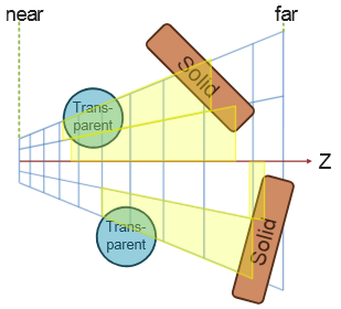 .
.
-
-
To improve on this we extend clustered forward shading by constructing the grid using a pre-pass over all geometry (not just opaque), and flagging clusters as a side effect. This allows us to quickly find the unique clusters used.
-
As clusters contain only space around actual samples that need shading, efficiency is much better.
-
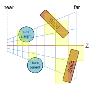 .
.
-
-
For deferred shading a single 1080p, 16x MSAA, 16-bit float RGBA buffer requires over 250Mb of memory. In addition, each sample may need to be shaded individually, effectively running shading at a per-sample frequency.
-
For forward shading, no G-Buffers are required and MSAA is trivially enabled.
Optimized Forward Renderer
-
High-level overview :
-
 .
.
-
-
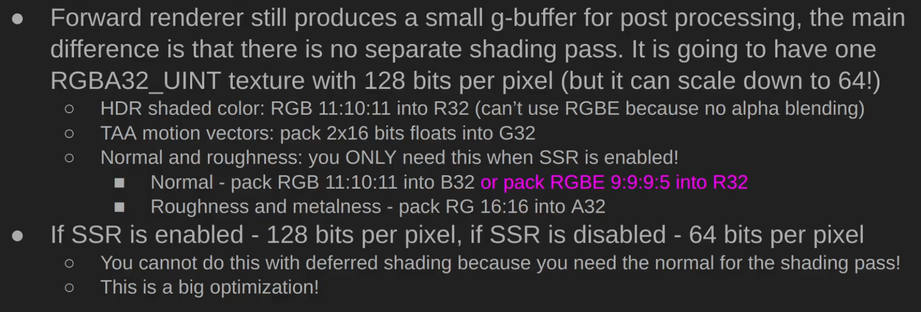 .
.
-
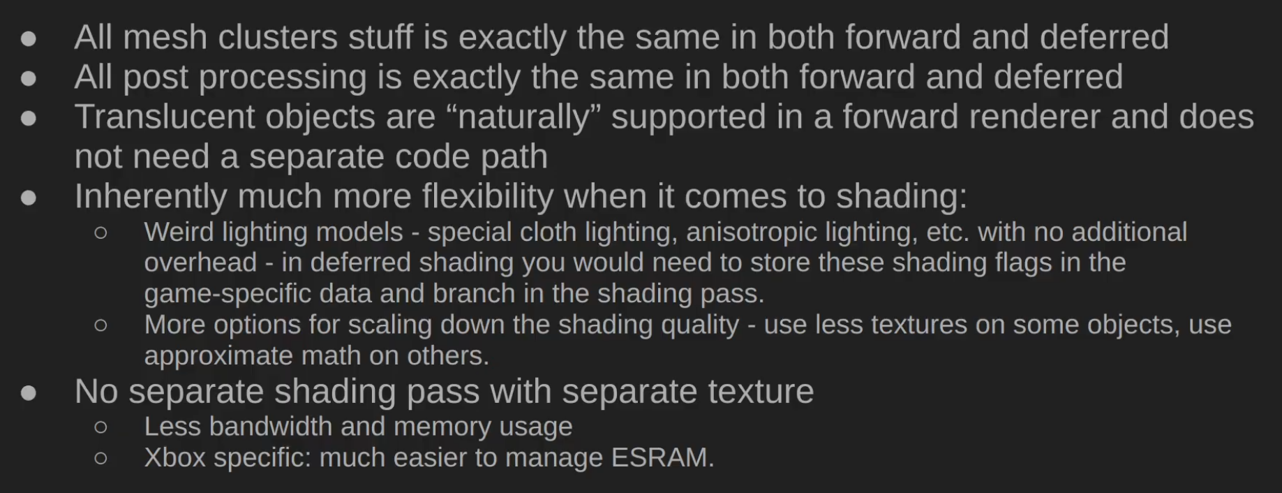 .
.
-
Performance caveats :
-
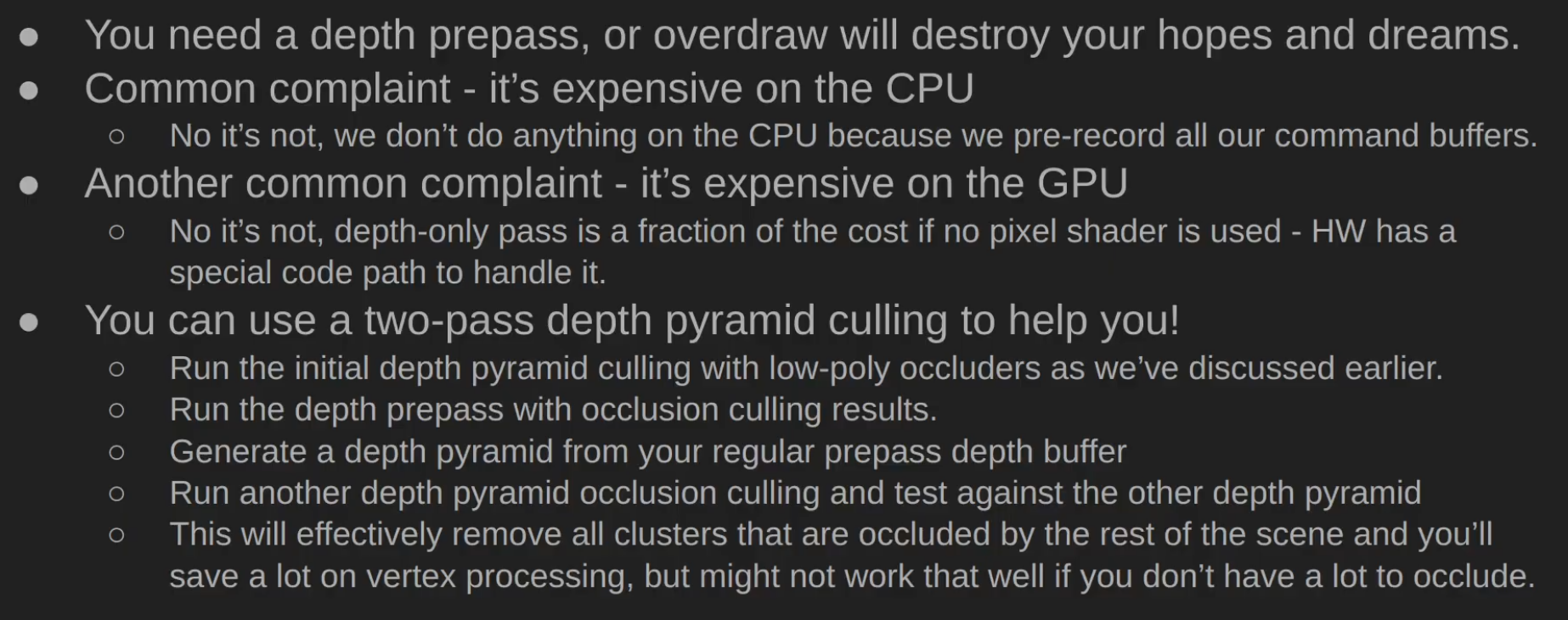 .
.
-
-
Triangle Overshading :
-
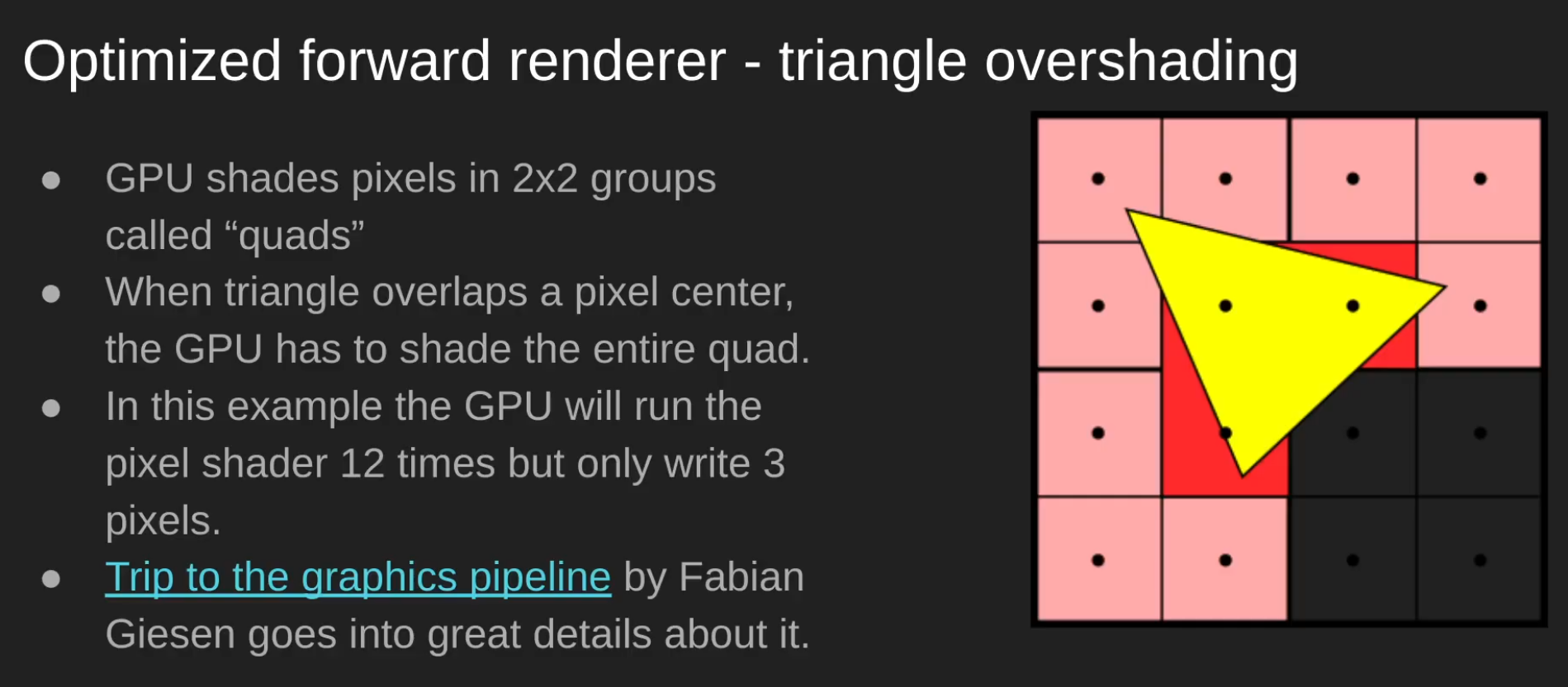 .
.
-
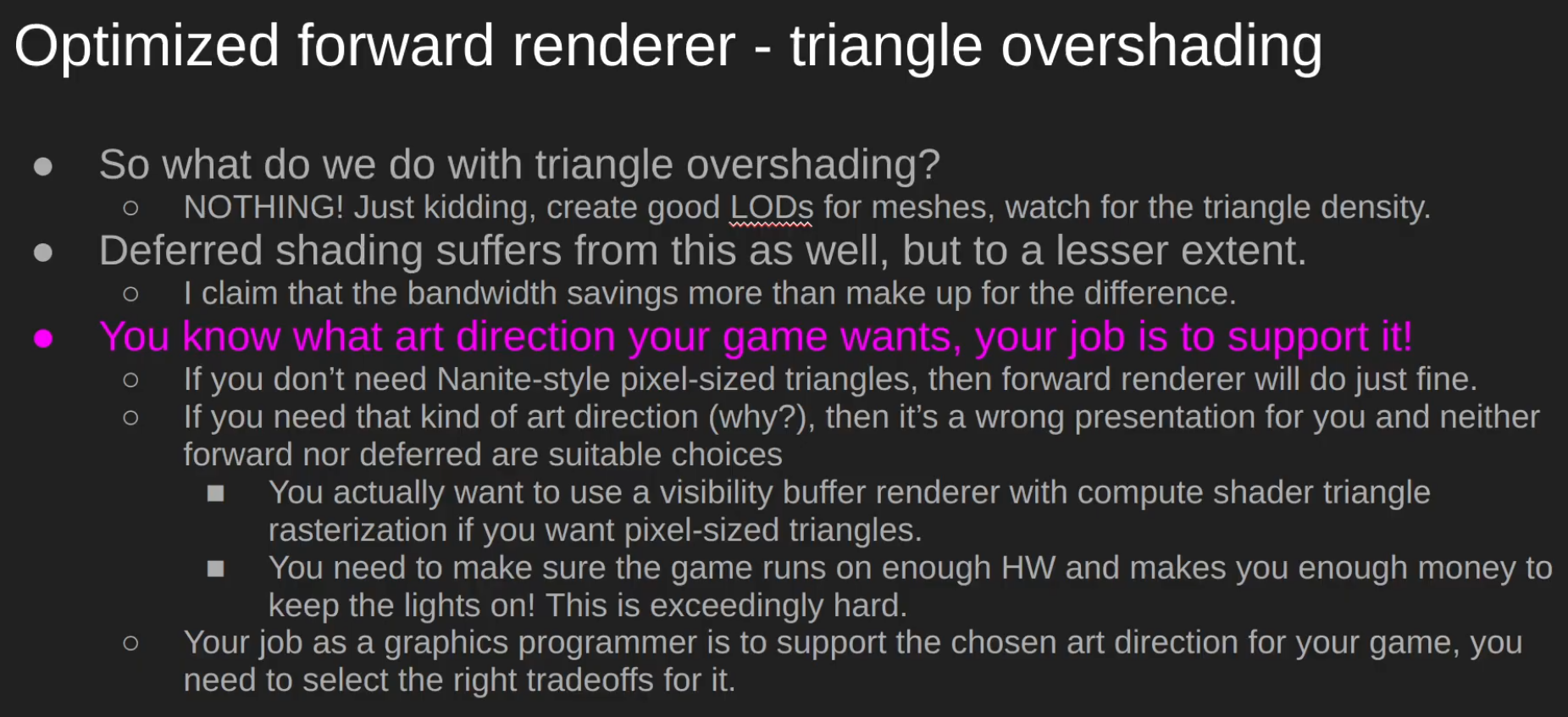 .
.
-
Papers and Presentations
-
Clustered Deferred and Forward Shading - Ola Olsson - 2012 .
-
Tiled and Clustered Forward Shading Supporting Transparency and MSAA - Ola Olsson - 2012 .
-
Efficient Real-Time Shading with Many Lights - Ola Olsson, Emil Persson (Avalanche) - 2014 .
-
Avalanche Studios did:
-
Just Cause 1 (Forward), Just Cause 2 (Forward), Mad Max (Deferred).
-
Just Cause 3, Just Cause 4, Generation Zero, Rage 2.
-
-
-
A Primer On Efficient Rendering Algorithms & Clustered Shading - Angel Ortiz - Rockstar North - 2018 .
-
Part 2 explains the implementation of the technique.
-
Great read, pretty good, with some implementation explanations and source code in OpenGL.
-
-
Cluster Shading OpenGL - David Hu - 2024 .
-
This is not a sample, just a C++ and OpenGL tutorial with some GLSL shaders for reference.
-
-
Clustered Forward Rendering and Anti-Aliasing in Detroit: Become Human - GDC 2018 .
-
~ Volume Tiled Forward Shading - Jeremiah Van Oosten - 2017 .
-
Supposedly: Volume > Clustered > Tiled.
-
Volume Tiled Forward Shading is based on Tiled and Clustered Forward Shading from Ola Olsson.
-
By first constructing a Bounding Volume Hierarchy (BVH) over the lights, we can achieve millions of light sources while maintaining real-time frame rates.
-
Impressions :
-
So... it seems the only thing he did was add BVH to the technique, however that seems to already be done by default in the culling part of Clustered Shading....
-
I don't understand. Did someone copy someone here? I'm confused...
-
His master's thesis is huge, but much of it is kind of "padding", as it's just a presentation of previous works.
-
Hmmm idk. He's not wrong, it just sounds odd.
-
-
-
Practical Clustered Shading - Avalanche Studios 2015.-
Exactly the same presentation as 'Efficient Real-Time Shading with Many Lights - Ola Olsson, Emil Persson (Avalanche) - 2014'; see that presentation, since it has presenter comments.
-
-
Practical Clustered Shading 2/4 - Avalanche Studios - 2014.-
The presentation comes after 'Efficient Real-Time Shading with Many Lights - Ola Olsson, Emil Persson (Avalanche) - 2014', since Just Cause 3 had already been announced, using Clustered Shading.
-
The presentation is very similar to 'Efficient Real-Time Shading with Many Lights - Ola Olsson, Emil Persson (Avalanche) - 2014'.
-
-
Managing many lights in real time with clustered shading - Ola Olsson 2016.-
Based on the 'Efficient Real-Time Shading with Many Lights - Ola Olsson, Emil Persson (Avalanche) - 2014' presentation, with basically no changes.
-
I preferred to read the former, for better slide visibility and because the presentation is much more in-depth. Also, the earlier presentation seemed to have more enthusiasm and depth; perhaps the audience for this presentation did not show much enthusiasm.
-
Samples
-
HybridRenderingEngine OpenGL (Clustered Forward/Deferred) - Sample - Angel Ortiz - 2018 .
-
Clustered Forward/Deferred Renderer
-
Physically Based shading
-
Image Based Lighting
-
Metallic workflow
-
Cook-Torrance specular BRDF (w/ lambert diffuse)
-
Ambient Occlusion & Emissive mapping
-
Tangent space normal mapping
-
HDR/linear lighting
-
HDR/LDR skyboxes
-
Exposure based tone mapping
-
Bloom
-
Multisample Anti-aliasing (MSAA)
-
Directional & point light sources
-
Compute shader based light culling
-
Alpha tested foliage (sponza atrium)
-
Directional light dynamic shadow mapping
-
Static Omnidirectional Shadow Mapping for Point Lights
-
Forward, Tiled Forward and Deferred rendering implementations
-
Located in other branches of the repo. Only clustered rendering is actively being developed.
-
-
Engine:
-
OpenGL 4.5+
-
SDL2 backend
-
JSON Parsing via Nlohmann: JSON for C++
-
Model Loading via ASSIMP (OBJ, FBX, gLTF2.0 etc)
-
Scene contents clearly outlined in JSON file
-
Multiple image loading paths via stb-image and GLI
-
Immediate mode GUI for debugging via ImGUI
-
Fully commented for future referencing
-
Environment map generation on load for IBL and skyboxes
-
Free flight camera
-
-
Deferred Shading
Deferred
-
Deferred shading is a screen-space shading technique that is performed on a second rendering pass, after the vertex and pixel shaders are rendered.
-
"I like to call it a "fake rendering", as at the end of the day you'll be just doing your shading on a quad, not on the geometry".
-
A shader that collects all geometry information into buffers, matches the first stage of a deferred renderer.
-
GBuffer ("Geometry Buffer") :
-
G-buffer is a set of textures or render targets used in deferred shading/rendering.
-
Instead of directly shading fragments during rasterization (as in forward rendering), the GPU first stores per-fragment data into the G-buffer.
-
A later pass (the lighting pass) reads from these buffers to compute lighting, shadows, reflections, etc.
-
A typical G-buffer contains attributes such as:
-
World/eye space position of the fragment
-
Normals
-
Albedo (base color)
-
Specular properties
-
Possibly depth, roughness, metalness, etc.
-
-
The key point is: the first pass writes geometry information into multiple render targets (the G-buffer), and the second pass consumes it for lighting.
-
-
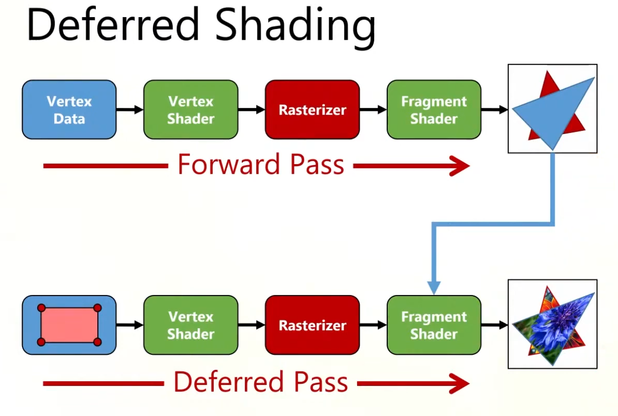 .
.
-
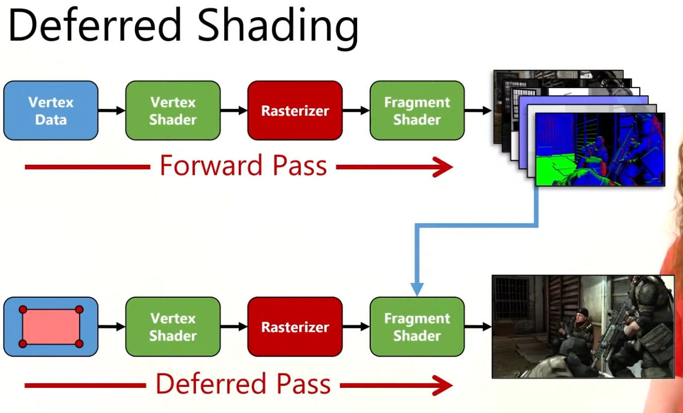 .
.
-
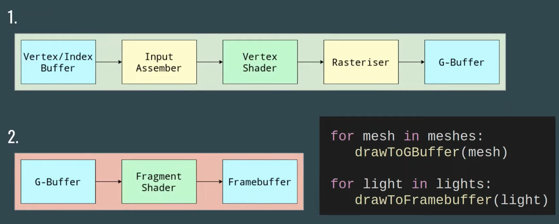 .
.
-
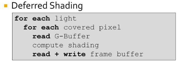 .
.
-
The problem is from the fact that the innermost loop is over the pixels.
-
This requires repeated reading and writing of the G-Buffers and frame buffer.
-
Disadvantages
-
Bandwidth :
-
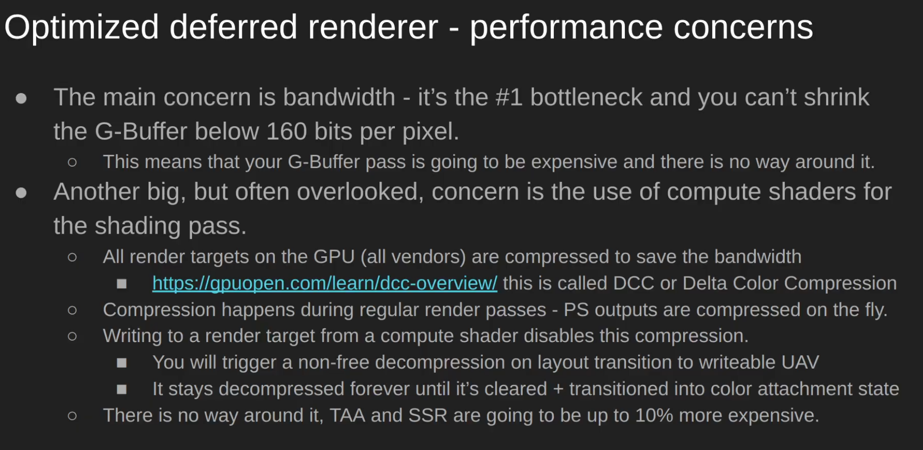 .
.
-
Consider marking non-persistent attachments as transient (
VK_ATTACHMENT_STORE_OP_DONT_CARE/ lazily allocated) so tile-based GPUs can keep them on-tile and reduce bandwidth.
-
-
Transparency :
-
Inability to handle transparency within the algorithm, although this problem is a generic one in Z-buffered scenes and it tends to be handled by delaying and sorting the rendering of transparent portions of the scene.
-
Depth peeling can be used to achieve order-independent transparency in deferred rendering, but at the cost of additional batches and g-buffer size.
-
Modern hardware, supporting DirectX 10 and later, is often capable of performing batches fast enough to maintain interactive frame rates.
-
When order-independent transparency is desired (commonly for consumer applications) deferred shading is no less effective than forward shading using the same technique.
-
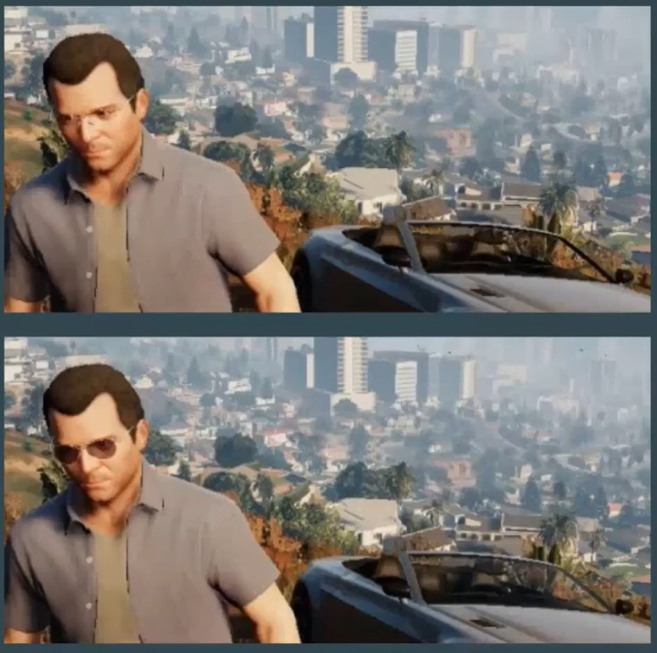 .
.
-
Example from GTA V.
-
-
Opaque is drawn with deferred renderer.
-
Transparent is drawn with forward renderer and then blended with the result of the deferred renderer.
-
-
Difficulty with using multiple materials :
-
It's possible to use many different materials, but it requires more data to be stored in the G-buffer, which is already quite large and takes up a large amount of the memory bandwidth.
-
Memory and bandwidth heavy (multiple render targets).
-
-
Another disadvantage of deferred shading is that only a single lighting model can be simulated in the lighting pass. This is due to the fact that it is only possible to bind a single pixel shader when rendering the light geometry. This is usually not an issue for pipelines that make use of übershaders as rendering with a single pixel shader is the norm, however if your rendering pipeline takes advantage of several different lighting models implemented in various pixel shaders then it will be problematic to switch your rendering pipeline to use deferred shading.
-
Bad MSAA :
-
Due to separating the lighting stage from the geometric stage, hardware anti-aliasing (MSAA) does not produce correct results anymore since interpolated subsamples would result in nonsensical position, normal, and tangent attributes.
-
One of the usual techniques to overcome this limitation is using edge detection (MLAA, FXAA, DLAA, or post MSAA) on the final image and then applying blur over the edges. TAA can also be used.
-
DirectX 10 introduced features allowing shaders to access individual samples in multi-sampled render targets (and depth buffers in version 10.1), giving users of this API access to hardware anti-aliasing in deferred shading. These features also allow them to correctly apply HDR luminance mapping to anti-aliased edges, where in earlier versions of the API any benefit of anti-aliasing may have been lost.
-
-
Extra complexity
-
G-buffer packing, formats, reconstructing positions, light culling systems, extra render passes and descriptor management.
-
Variants
-
As said by Ola Olsson:
-
Deferred Lighting
-
Factor out specular and diffuse color.
-
G-Buffer only stores normal and shininess.
-
Output diffuse and specular shading.
-
Second geometry pass which multiple colors.
-
-
Light Prepass.
-
Much like the above.
-
But with monochromatic specular highlight.
-
-
They offer similar performance as deferred.
-
Only improves constant factors.
-
Limits shading model even further.
Tiled Deferred
-
Tiled deferred shading removes the bandwidth bottleneck from deferred shading, instead making the technique compute bound. This enables efficient usage of devices with a high compute-to-bandwidth ratio, such as modern consoles and GPUs. Modern high-end games are using tiled deferred shading to allow for thousands of lights, which are required to push the limits of visual fidelity.
-
With large numbers of lights, GI effects can be produced that affect dynamic as well as static geometry.
-
Steps:
-
Render scene to G-Buffers.
-
Cluster assignment.
-
Find unique clusters.
-
Assign lights to clusters.
-
Shade samples.
-
-
The first step, rendering the model to populate the G-Buffers, does not differ from traditional deferred shading or from tiled deferred shading. The second step computes for each pixel which cluster it belongs to according to its position (possibly normal). In the third step, we reduce this into a list of unique clusters. The fourth step, assigning lights to clusters, consists of efficiently finding which lights influence which of the unique clusters and produce a list of lights for each cluster. Finally, for each sample, these light lists are accessed to compute the sample’s shading.
-
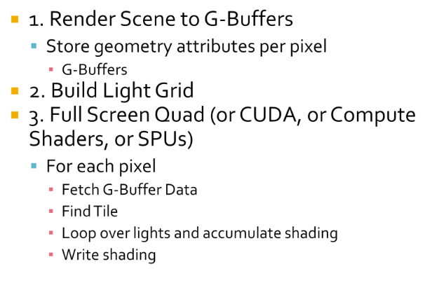 .
.
-
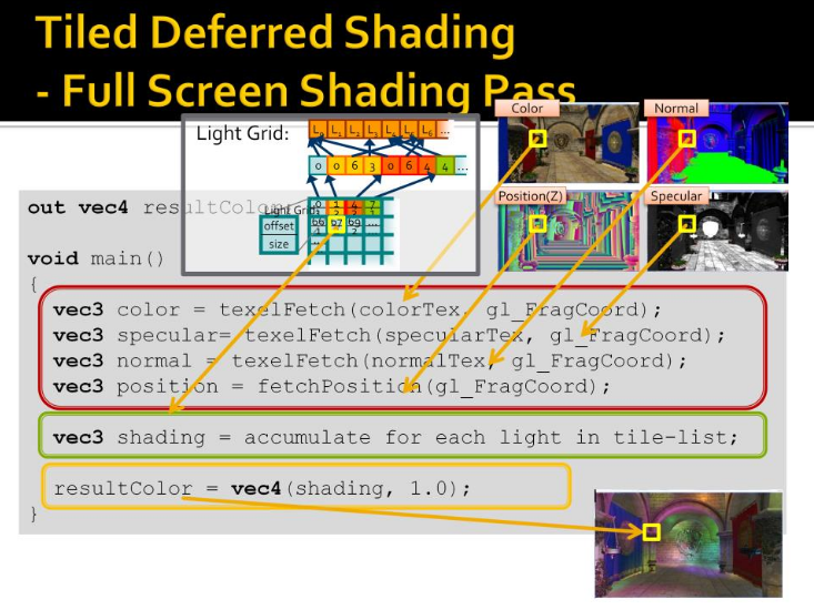 .
.
-
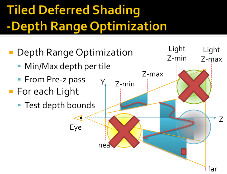 .
.
-
Tiles in 1D, from side
-
View Frustum
-
4 subdivisions
-
Redline is geometry
-
Min and max depth per tile
-
Light range, rejected, completely hidden
-
Another rejected, completely in front
-
Rejected in one tile, not others
-
Usage
-
Uncharted: Drake’s fortune.
-
Battlefield 3.
-
PlayStation 3.
-
Xbox 360.
Optimized Deferred Renderer
-
High-level overview :
-
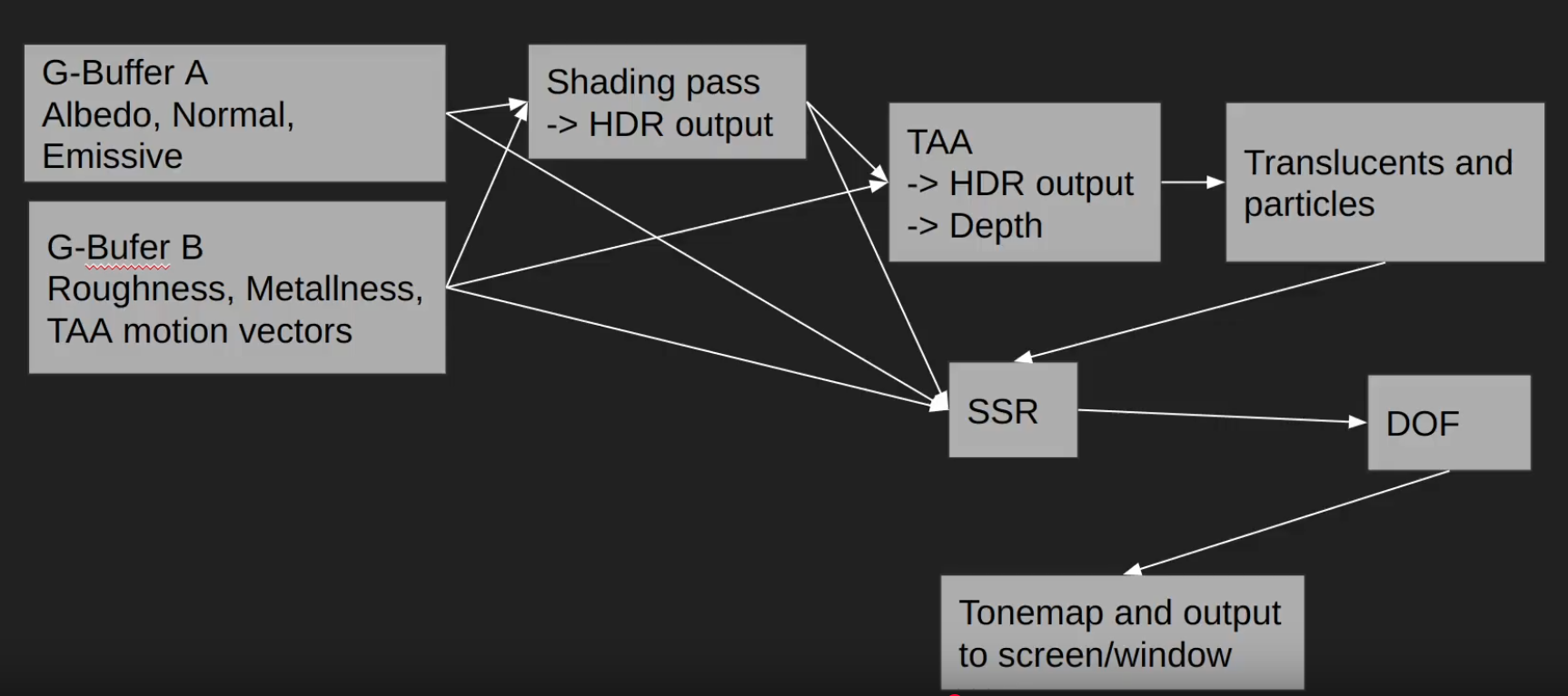 .
.
-
For SSR you need to take a lot of samples from G-Buffer B, and one sample from the shading color from the TAA pass.
-
We do the Raymarching using roughness and depth, once that is done we sample the TAA to get the final color.
-
-
DOF: Depth of Field.
-
-
-
Compressing the GBuffer
-
Optimized deferred shading renderer:
-
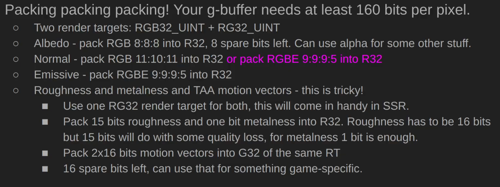 .
.
-
Random person in the comments: There's a small typo - Normal should be G32 and Emissive should be B32.
-
Does it make sense? maybe?
-
-
-
-
Lights :
-
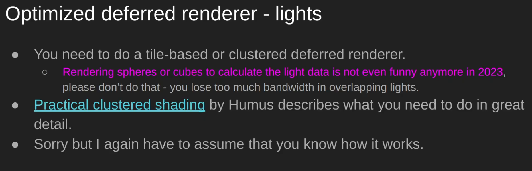 .
.
-
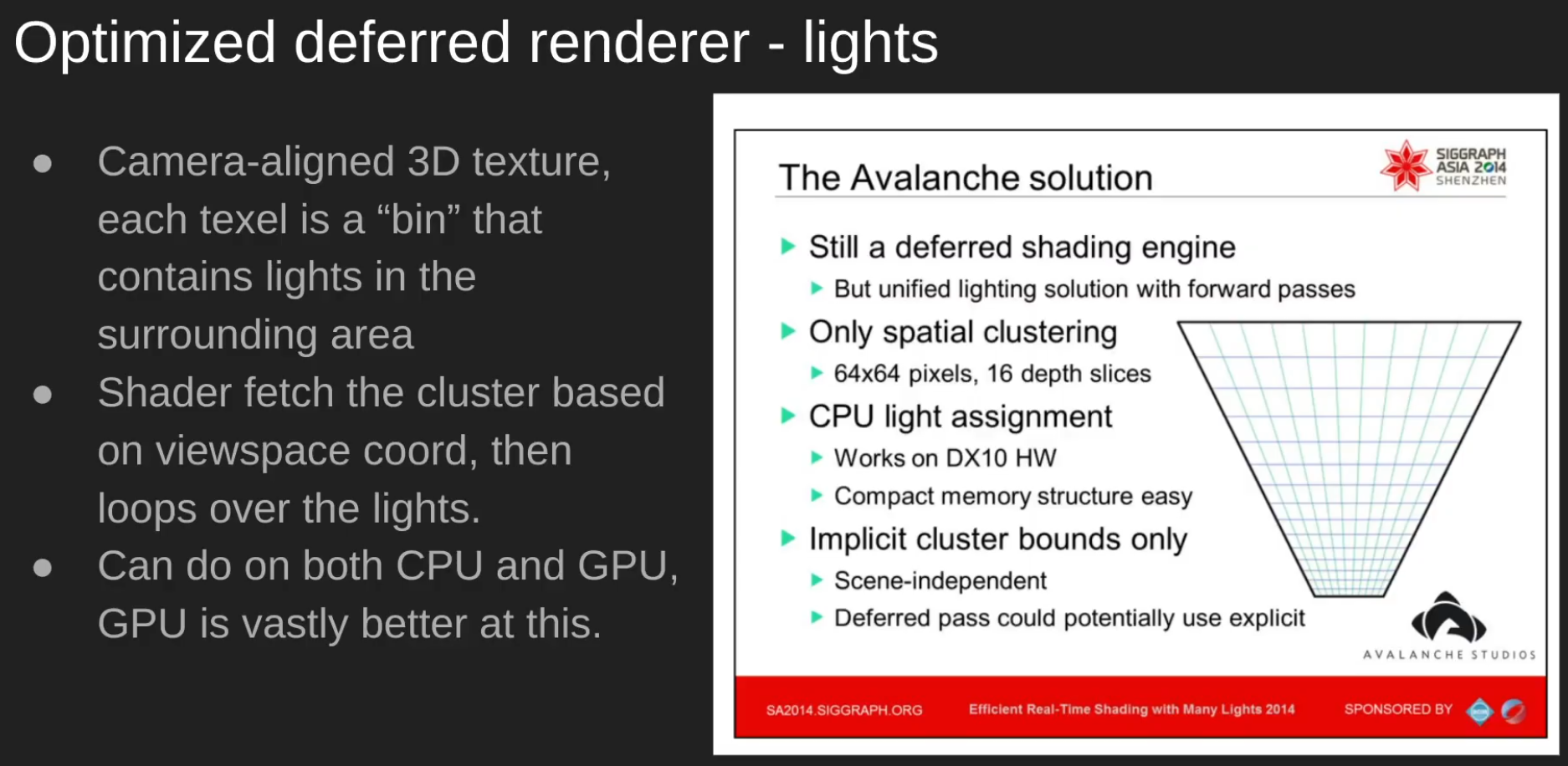 .
.
-
-
Decals :
-
 .
.
-
Clustered Decals > D-Buffer.
-
-
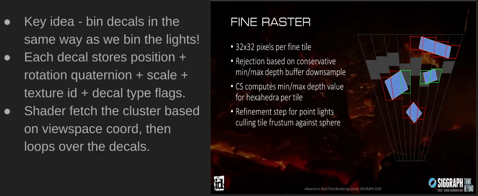 .
.
-
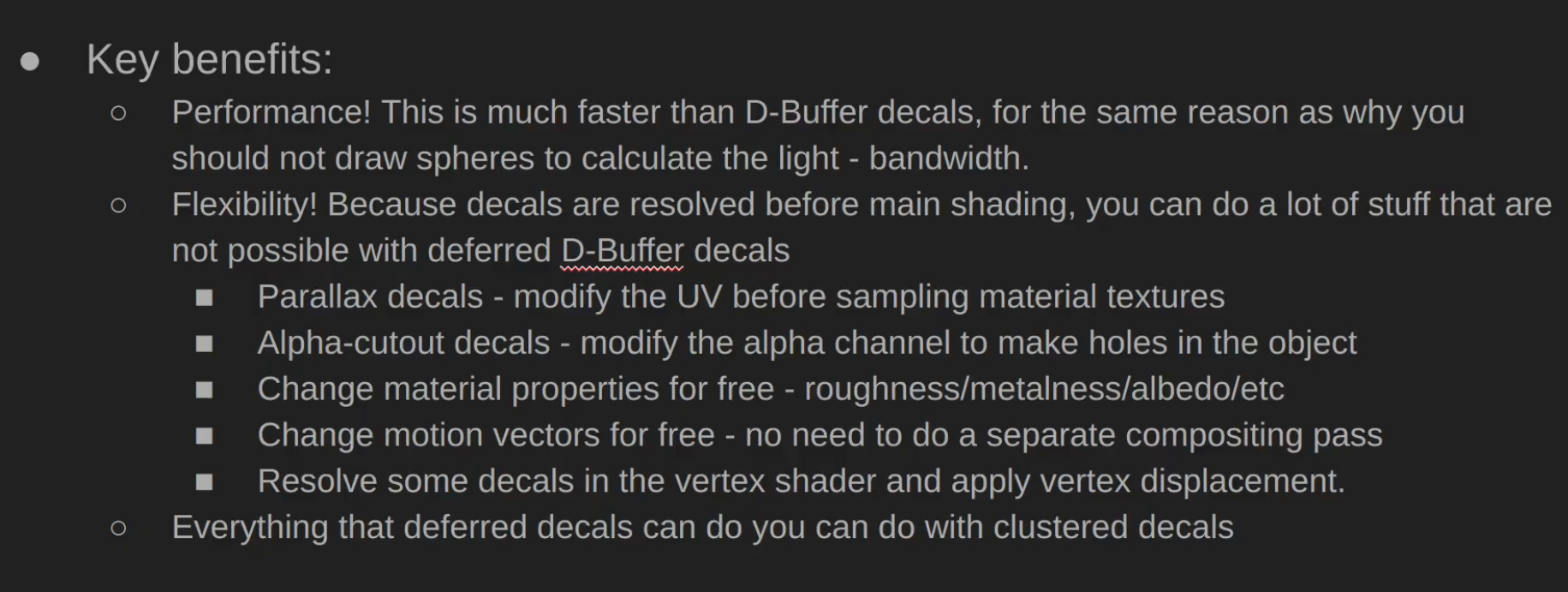 .
.
-
-
Post-processing :
-
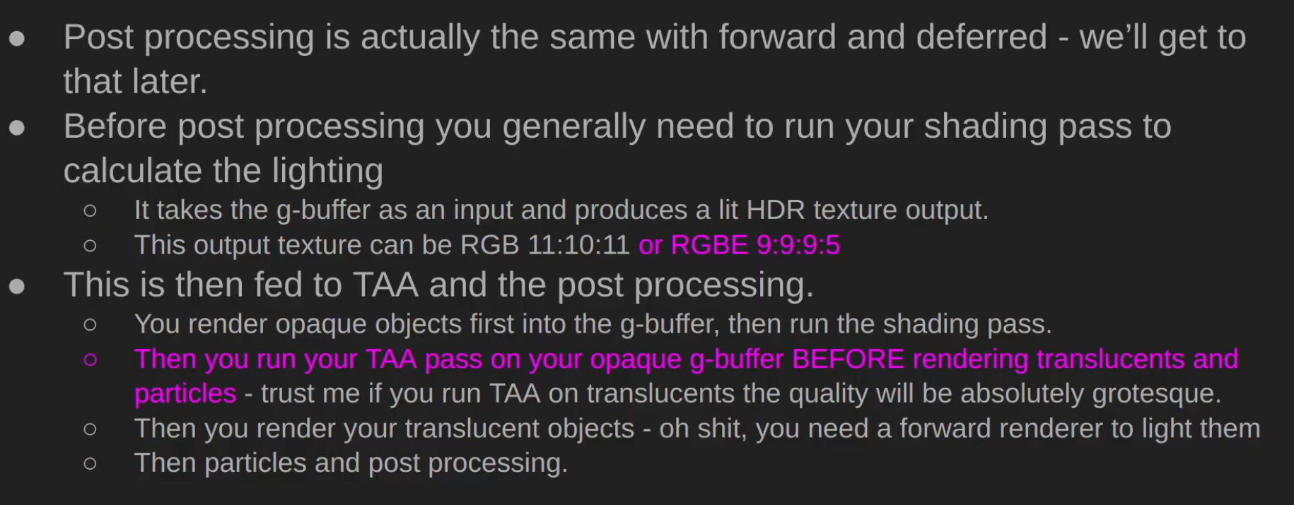 .
.
-
-
Demo and Source Code - Sascha Willems .
-
Based on my deferred shading example this new example adds shadows from multiple spotlights using shadow mapping. To avoid having multiple render passes for rendering the scene's depth from each of the light's point-of-view the example uses a layered depth attachment and multiple geometry shader invocations, so that an arbitrary number of depth maps can be generated in one pass. Each layer in the attachment corresponds to a light source and the geometry shader does multiple invocations on each vertex to output the scene into the different layers of the attachment. Each invocation uses a different light's mvp matrix. The final scene compositing pass then samples from the depth map array texture to determine if a fragment is shadowed or not.
-
-
Demo .
-
"Deferred lighting is physically based, using Cook-Torrance as the BRDF. In this demo the forward pass is only responsible for drawing the skybox, but could draw other rasterization pipelines not suitable for the deferred passes."
-
-
Demo .
-
Jonathan Blow's criticisms of Deferred Rendering .
-
He bullshits and claims it's bad, unjustifiable.
-
"Doesn't make sense in the modern day".
-
Counter-argument:
-
Deferred is defined very very simply - do you have a G-buffer? If the answer is yes - you're deferred.
-
Pretty much all of high-performance forward renderers do a "depth pre-pass", which is sort-of like "deferred lite".
-
Forward has a huge benefit of being very bandwidth efficient, but it's very compute inefficient.
-
About transparencies - transparency is hard. Most forward renderers suck at transparency, most deferred suck as well. Forward makes it a bit easier, because your architecture is about the same.
-
About lighting, Jonathan Blow clearly is not a graphics engineer, there's tiled and clustered rendering that has existed since late 2000s which is typically called Forward+, same techniques are used in deferred, but hey man... the whole lighting argument is over a decade out of date.
-
-
Counter-argument:
-
Deferred solves the problem of doing the pricey per-pixel calculations only on the pixels that will be visible in the end result. Which is why, contrary to what he said, basically every engine went deferred. I like the guy but this is maybe the worst take that I've ever heard him say? He doesn't really get why it's used AND he is wildly off the mark about its popularity in general. If anything, forward had a pretty big comeback with phones and VR.
-
-
Pro argument:
-
Deferred rendering is an optimization technique to make lighting cheaper, but has massive complexity, VRAM, and image quality downsides. There's not really an upside besides being cheap to process many lights. There's a few ultra high end games that are slowly ditching deferred for forward+ systems. I think in a few years there's a good chance deferred won't be common. Even if raytracing doesn't happen.
-
-
Counter-argument:
-
Forward+ still doesn't solve the problem of shadow casting lights. Deferred at least has lower overhead, so the bits of computing power go to shadow mapping purposes.
-
-
Clustered Deferred
-
Avalanche Studios :
-
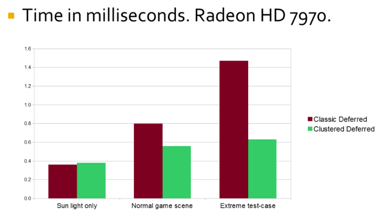 .
.
-
Adaptive Deferred Shading
-
It's a selective way to choose what to perform shading on.
-
He compared it with VRS while using deferred shading.
Optimization Techniques
Shader Branching
-
Math is faster than branching with control flow.
-
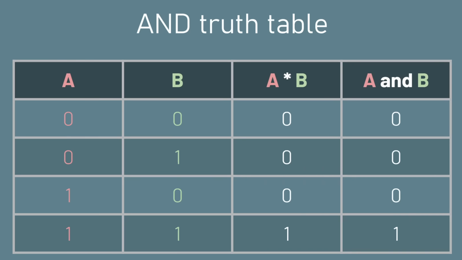 .
.
-
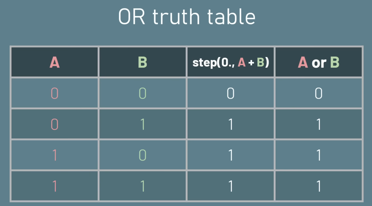 .
.
-
 .
.
AZDO (Approach Zero Driver Overhead)
Motivation
-
GPUs have orders of magnitude higher performance than CPU on data-parallel algorithms. Rendering is almost all data parallel algorithms.
-
With the GPU deciding its own work, latencies are minimized as there is no roundtrip from CPU to GPU and back.
-
Frees up the CPU from a lot of work which can now be used on other things.
-
Repeated small
vkCmdBindVertexBuffers/vkCmdBindIndexBufferandvkCmdDrawIndexedcalls force the driver to record many small draw commands (and possibly do relocations or check memory), which is expensive. -
Many small state changes cause the driver to update internal tables, validate, or patch commands — that’s CPU work and cannot be avoided without batching.
-
Different drivers / GPUs behave differently. Some drivers do more CPU work per bind/draw and will be worse in this pattern.
-
Query commands from a GPU buffer. This has two significant advantages:
-
Draw calls can be generated from the GPU (such as in a "compute shader"), and
-
An array of draw calls can be called at once, reducing command buffer overhead
-
Optimizations
-
Batch
vkCmdDrawIndexed: Multi-draw Indirect.-
vkCmdDrawIndexedIndirect/ multi-draw indirect to let GPU consume a small indirect buffer with many draws in one driver call. -
Avoid binding vertex/index buffer per draw — bind the quad vertex/index buffer once and supply per-instance data via instance attributes or an SSBO.
-
-
Batch
vkCmdPushConstants.-
(2025-12-01) From 5 push calls taking 7.65us, to now 1 push call taking 3.08us.
-
-
Batch
vkCmdBindDescriptorSets: using Bindless.-
Bindless Textures.
-
Bindless / descriptor indexing (
VK_EXT_descriptor_indexing/ descriptor arrays with update-after-bind) so you can bind a single descriptor set containing all textures and index into it in the shader using the per-instance texture index. This removes the per-drawvkCmdBindDescriptorSets. -
Binding a descriptor set per draw is heavy if each set references different image samplers; the driver must ensure the GPU has correct descriptors ready (or patch them).
-
-
Batch textures: Texture Atlas.
-
Pack multiple textures into atlases or a texture array and index into them.
-
-
Pre-record commands.
-
Useful if CPU-bound.
-
-
GPU Culling:
-
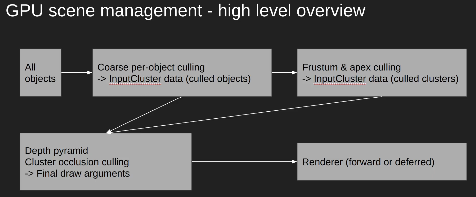 .
.
-
All culling passes would be a single pass, for performance reasons.
-
Etc
-
Once we have a renderer where everything is stored in big GPU buffers, and we don’t use PushConstants or descriptor sets per object, we are ready to go with a GPU-driven-renderer.
-
Because it takes its parameters from a buffer, it is possible to use compute shaders to write into these buffers and do culling or LOD selection in compute shaders. Doing culling this way is one of the simplest and most performant ways of doing culling. Due to the power of the GPU you can easily expect to cull more than a million objects in less than half a millisecond. Normal scenes don’t tend to go as far. In more advanced pipelines like the one in Dragon Age or Rainbow Six, they go one step further and also cull individual triangles from the meshes. They do that by writing an output Index Buffer with the surviving triangles and using indirect to draw that.
-
Store the matrices for all loaded objects into a big SSBO. In GPU driven pipelines, we also want to store more data, such as material ID and cull bounds.
-
GPU driven pipelines work best when the amount of binds is as limited as possible. Best case scenario is to do a extremely minimal amount of BindVertexBuffer, BindIndexBuffer, BindPipeline, and BindDescriptorSet calls.
-
The less drawcalls you use to render your scene, the better, as modern GPUs are really big and have a big ramp up/ramp down time. Big modern GPUs love when you give them massive amounts of work on each drawcall, as that way they can ramp up to 100% usage.
-
The new Unreal 5 engine relies heavily on compute shaders for software rasterization.
-
The first thing is to go all in on object data in GPU buffers. Per-object PushConstants are removed, per-object dynamic uniform buffers are removed, and everything is replaced by ObjectBuffer where we store the object matrix and we index into it from the shader.
-
A Batch is a set of objects that matches material and mesh. Each batch will be rendered with one DrawIndirect call that does instanced drawing. Each mesh pass (forward pass, shadow pass, others) contains an array of batches which it will use for rendering.
-
When starting the frame, we sync the objects that are on each mesh pass into a buffer. This buffer will be an array of ObjectID + BatchID. The BatchID maps directly as an index into the batch array of the mesh-pass.
-
Once we have that buffer uploaded and synced, we execute a compute shader that performs the culling.
-
For every object in said array of ObjectID + BatchID pairs, we access the object data in the ObjectBuffer using the ObjectID, and check if it is visible. If it’s visible, we use the BatchID index to insert the draw into the Batches array, which contains the draw indirect calls, increasing the instance count. We also write it into the indirection buffer that maps from the instance ID of each batch into the ObjectID.
-
With that done, on the CPU side we iterate over the batches in a mesh pass, and execute each of them in order, making sure to bind each batch pipeline and material descriptor set. The gpu will then use the parameters it just wrote into from the culling pass to render the objects.
-
Buffer Storage.
-
Direct State Access.
-
Shader Buffer Load.
-
UBO & SSBO.
-
and more...
Avoid being Vertex Bound
-
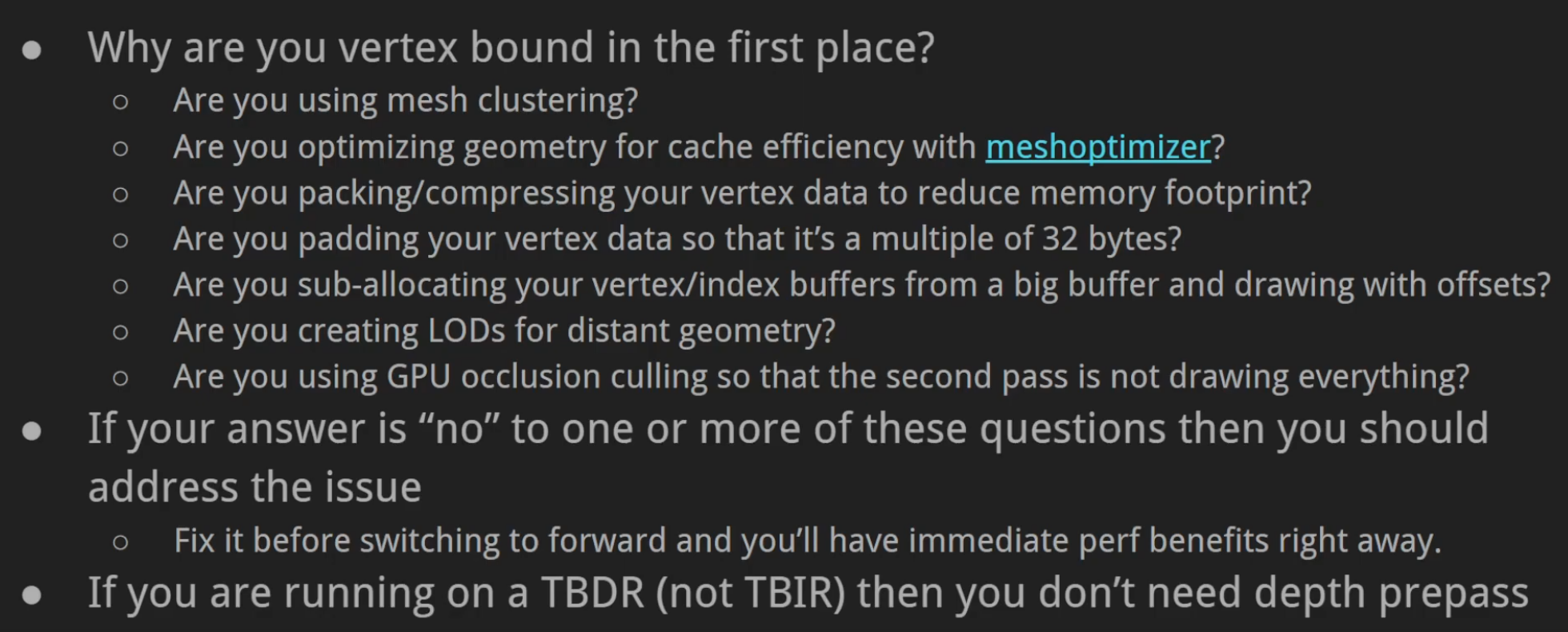 .
.
-
TBDR: Tile Based Deferred Renderer GPU.
-
TBIR: Tile Based Immediate Renderer GPU.
-
-
-
When a GPU renders triangle meshes, various stages of the GPU pipeline have to process vertex and index data. The efficiency of these stages depends on the data you feed to them; this library provides algorithms to help optimize meshes for these stages, as well as algorithms to reduce the mesh complexity and storage overhead.
-
The library provides a C and C++ interface for all algorithms; you can use it from C/C++ or from other languages via FFI (such as P/Invoke).
-
gltfack .
-
gltfpack is a tool that can automatically optimize glTF files to reduce the download size and improve loading and rendering speed.
-
-
Instancing
-
Billboard Grass and GPU Instancing .
-
"Rendering millions of grass".
-
The video is cool.
-
We'll use a compute shader.
-
We take the thread id of our compute shader thread. For a 300 square space, we can do
position = id.xy - 150so it's centered over the origin. -
As our grass is made of 3 meshes (3 billboard quads), this will result in 3 separate instancing calls.
-
To increase the density of grasses in the square space, we can
position *= (1 / density); I'll usedensity = 2. -
For this example, I'll render 2,160,000 triangles at 523 fps.
-
Screen: 1289x621
-
Setup? GTX 1660, apparently.
-
-
To get randomness, I did
pos.xz += noise()for the position andposition.y += noise()to get a different height (higher grass will be grouped with higher grasses).-
This uses a simplex noise.
-
-
To animate, I'll just skew the top 2 vertices of the mesh in the vertex shader.
-
{9:20} Explanation of what was done to randomize the intensity and frequency of grass sway movement.
-
Hash the instance id to get a hash id. With the hash_id, we check against a threshold to know if we perform a fast cosine or a slow cosine.
-
The grass height changed the cosine frequency.
-
Etc.
-
-
To get the grass displaced with the terrain displacement, we convert the space coordinates of our grass to uv coordinates, such as they can sample the same height map as the terrain mesh.
-
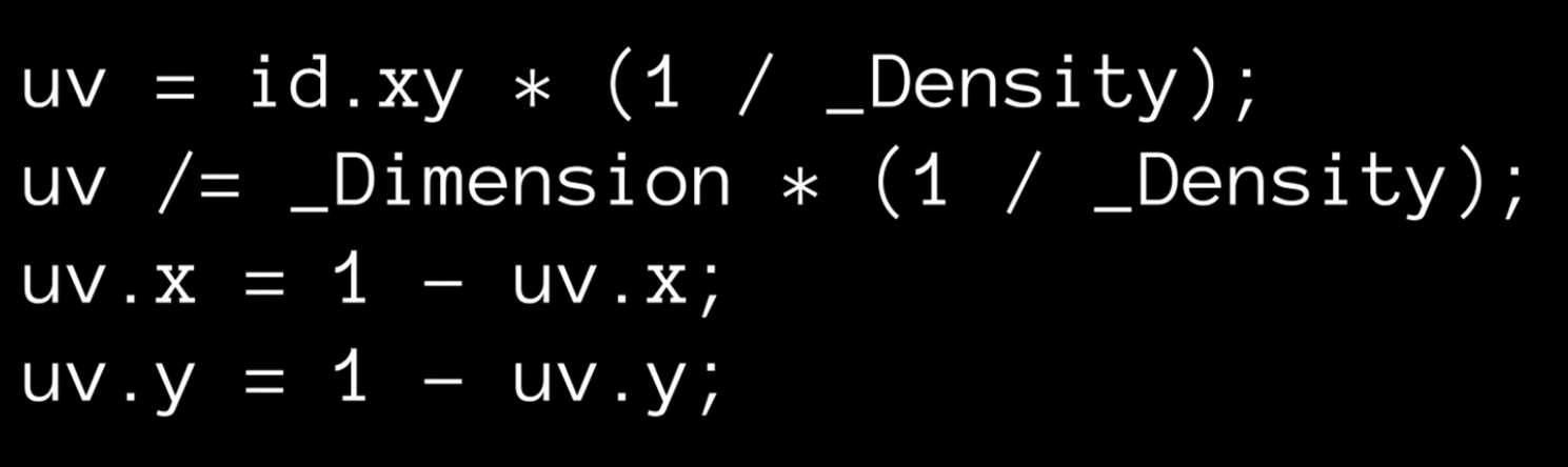 .
.
-
-
I also introduced a color variance in the grass, by making the tip of the grass more yellow, to show aging of the grass. This affects higher grasses a bit more, as they are older.
-
Continuation: Grass Mesh instead of Billboarding and GPU Culling with the Scan and Compact technique .
-
The video is the continuation of the previous one, changing: noise texture for wind simulation and optimizations with frustum culling with Scan and Compact.
-
The video is cool, though it has less content than the previous one.
-
It shows no implementation or formulas.
-
-
Noise is used for wind movement, more sophisticated using a noise texture with oscillations ~etc, different from the randomization used in the billboarding solution.
-
Then, optimization is discussed. This new technique is much heavier than the previous, so he uses Frustum Culling to optimize what is actually instanced.
-
This frustum culling apparently is harder to do, because it requires the Compute Buffer array to be contiguous.
-
He uses: Scan and Compact.
-
The array is scanned, marked for modification and a new array is created with the desired elements.
-
For this, a Prefix Sum Scan is used to define which entries form the new array.
-
This is not explained.
-
-
-
-
Continuation: LOD with Chunking .
-
The video is quite short, only talking about the optimization below. It shows no implementation or formulas.
-
It uses a mesh with lower poly count when the object's distance to the camera is greater than a threshold.
-
The justification for using chunking is to help with LOD.
-
Apparently LOD would be done in chunks (?) which would reduce the need for having a second position buffer, specific to the low-poly LOD mesh.
-
-
The final performance is 110fps, with 408MB of VRAM.
-
-
Scene Management
-
Google "GPU Scene Management" for some ideas - BVH, scene graph, ECS on the GPU, etc.
-
It has a concept of an "object" that users can place in the world.
-
These objects can contain multiple meshes and have a bounding box.
-
There is hierarchy (refer to flecs queries on how to do it efficiently).
-
Streaming is handled.
Culling
-
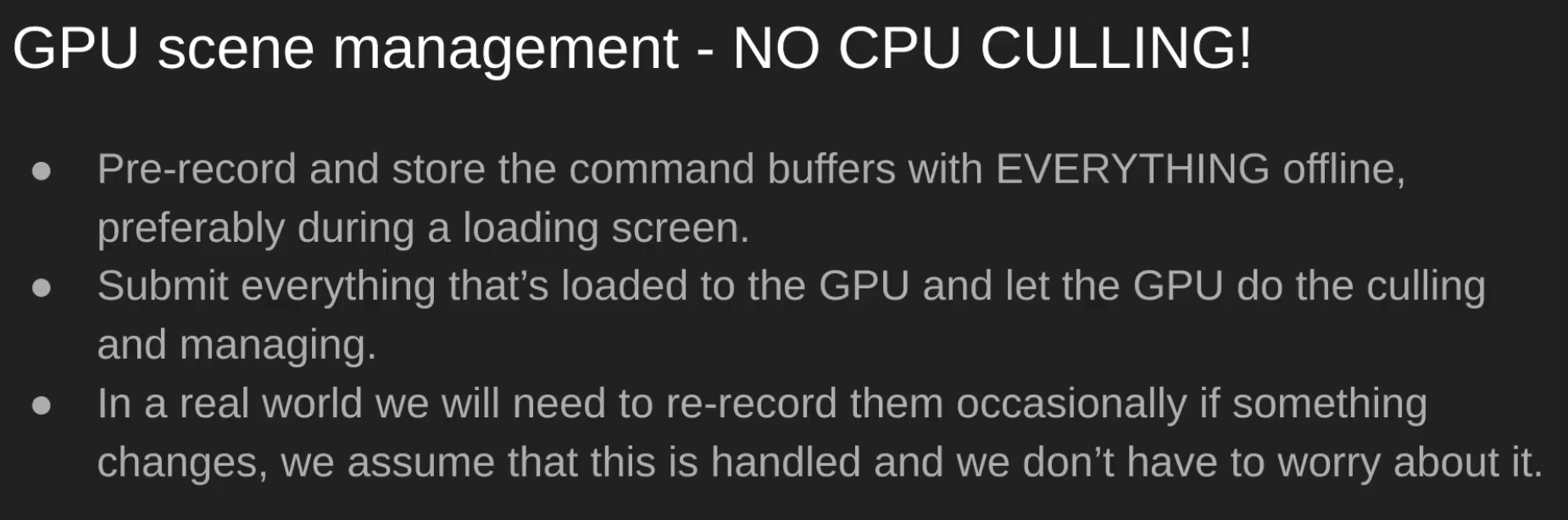 .
.
-
 .
.
Culling
-
Hierarchical Z-Buffer Culling - 2010 .
-
Rendering with Conviction - GDC 2010 presented this technique, which was first introduced on Siggraph 2008.
-
Hierarchical Z-Buffer Culling - Generating Occlusion Volumes - 2011 .
-
Frustum Culling
-
Tessellation Shader with LOD, Frustum Culling in the Geometry Shader .
-
The video is pretty cool, but shows absolutely no code or formulas. It's only a theoretical discussion of the techniques.
-
Creating geometry in the tessellation shader is better than passing the mesh on the GPU.
-
Data communication between CPU and GPU will always be the bottleneck.
-
This is not that precise, as the performance can actually be worse.
-
The real performance gain comes from tessellating based on the distance of the object, by using LOD; if it's far away, tessellate less.
-
-
The Frustum Culling is based on the bounding box of the mesh, but as the mesh is too big, we are always rendering every triangle of the mesh, even for triangles we don't see.
-
The Geometry Shader can finalize the geometry, as well as culling the triangles we don't need.
-
This technique is usually used for terrain, as it's displaced by a height map.
-
For characters, you would use different models with different poly count, rendering the correct one based on the distance to the camera.
-
-
CPU Frustum Culling :
-
The way this works is that we transform each of the 8 corners of the mesh-space bounding box into screen space, using the object matrix and view-projection matrix. From those, we find the screen-space box bounds, and we check if that box is inside the clip-space view. This way of calculating bounds is on the slow side compared to other formulas, and can have false-positives where it thinks objects are visible when they aren't. All the functions have different tradeoffs, and this one was selected for code simplicity and parallels with the functions we are doing on the vertex shaders.
-
We check for visibility before drawing.
bool is_visible(const RenderObject& obj, const glm::mat4& viewproj) { std::array<glm::vec3, 8> corners { glm::vec3 { 1, 1, 1 }, glm::vec3 { 1, 1, -1 }, glm::vec3 { 1, -1, 1 }, glm::vec3 { 1, -1, -1 }, glm::vec3 { -1, 1, 1 }, glm::vec3 { -1, 1, -1 }, glm::vec3 { -1, -1, 1 }, glm::vec3 { -1, -1, -1 }, }; glm::mat4 matrix = viewproj * obj.transform; glm::vec3 min = { 1.5, 1.5, 1.5 }; glm::vec3 max = { -1.5, -1.5, -1.5 }; for (int c = 0; c < 8; c++) { // project each corner into clip space glm::vec4 v = matrix * glm::vec4(obj.bounds.origin + (corners[c] * obj.bounds.extents), 1.f); // perspective correction v.x = v.x / v.w; v.y = v.y / v.w; v.z = v.z / v.w; min = glm::min(glm::vec3 { v.x, v.y, v.z }, min); max = glm::max(glm::vec3 { v.x, v.y, v.z }, max); } // check the clip space box is within the view if (min.z > 1.f || max.z < 0.f || min.x > 1.f || max.x < -1.f || min.y > 1.f || max.y < -1.f) { return false; } else { return true; } } -
-
VkGuide:
-
The instanceBuffer is AllocatedBuffer
instanceBuffer; from the last article. It stores ObjectID + BatchID (draw indirect ID)
bool IsVisible(uint objectIndex) { //grab sphere cull data from the object buffer vec4 sphereBounds = objectBuffer.objects[objectIndex].spherebounds; vec3 center = sphereBounds.xyz; center = (cullData.view * vec4(center,1.f)).xyz; float radius = sphereBounds.w; bool visible = true; //frustrum culling visible = visible && center.z * cullData.frustum[1] - abs(center.x) * cullData.frustum[0] > -radius; visible = visible && center.z * cullData.frustum[3] - abs(center.y) * cullData.frustum[2] > -radius; if(cullData.distCull != 0) {// the near/far plane culling uses camera space Z directly visible = visible && center.z + radius > cullData.znear && center.z - radius < cullData.zfar; } visible = visible || cullData.cullingEnabled == 0; return visible; } void main() { uint gID = gl_GlobalInvocationID.x; if(gID < cullData.drawCount) { //grab object ID from the buffer uint objectID = instanceBuffer.Instances[gID].objectID; //check if object is visible bool visible = IsVisible(objectID); if(visible) { //get the index of the draw to insert into uint batchIndex = instanceBuffer.Instances[gID].batchID; //atomic-add to +1 on the number of instances of that draw command uint countIndex = atomicAdd(drawBuffer.Draws[batchIndex].instanceCount,1); //write the object ID into the instance buffer that maps from gl_instanceID into ObjectID uint instanceIndex = drawBuffer.Draws[batchIndex].firstInstance + countIndex; finalInstanceBuffer.IDs[instanceIndex] = objectID; } } } -
Cluster
-
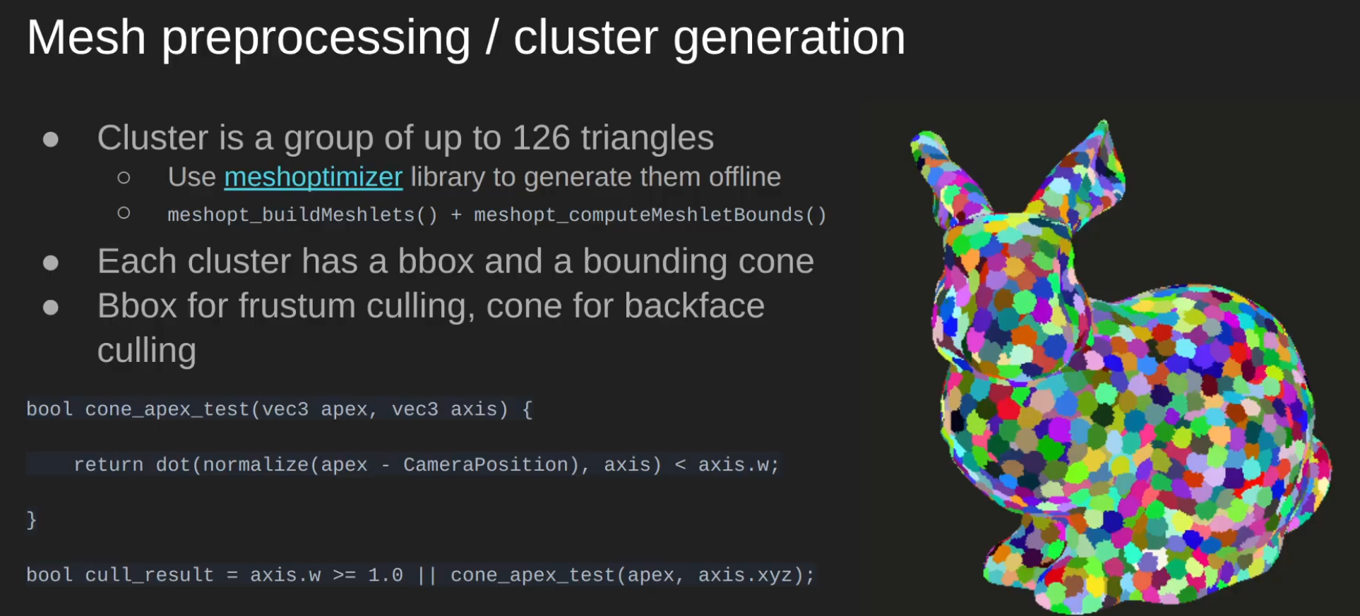 .
.
-
Each cluster is up to 64 vertices / 124 triangles.
-
-
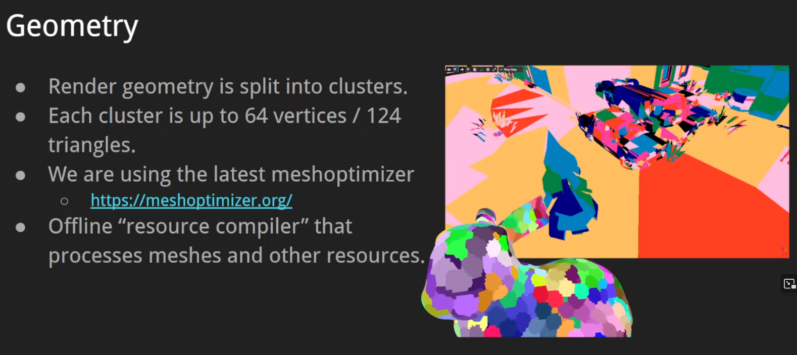 .
.
-
 .
.
-
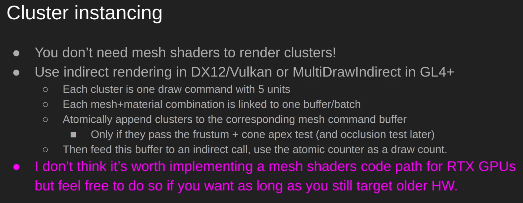 .
.
-
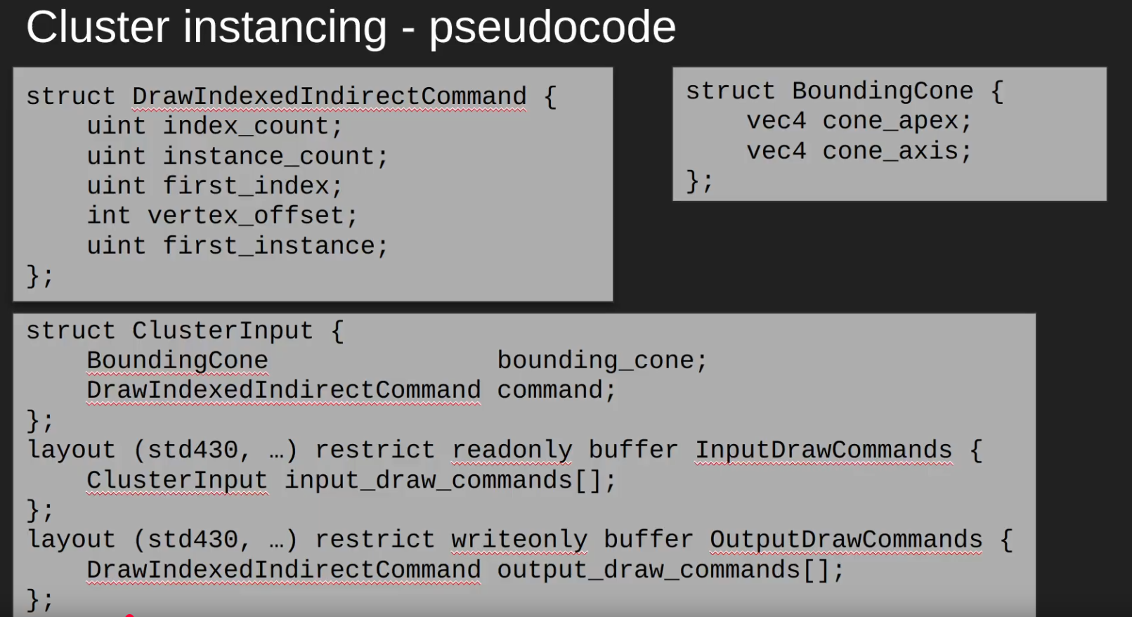 .
.
-
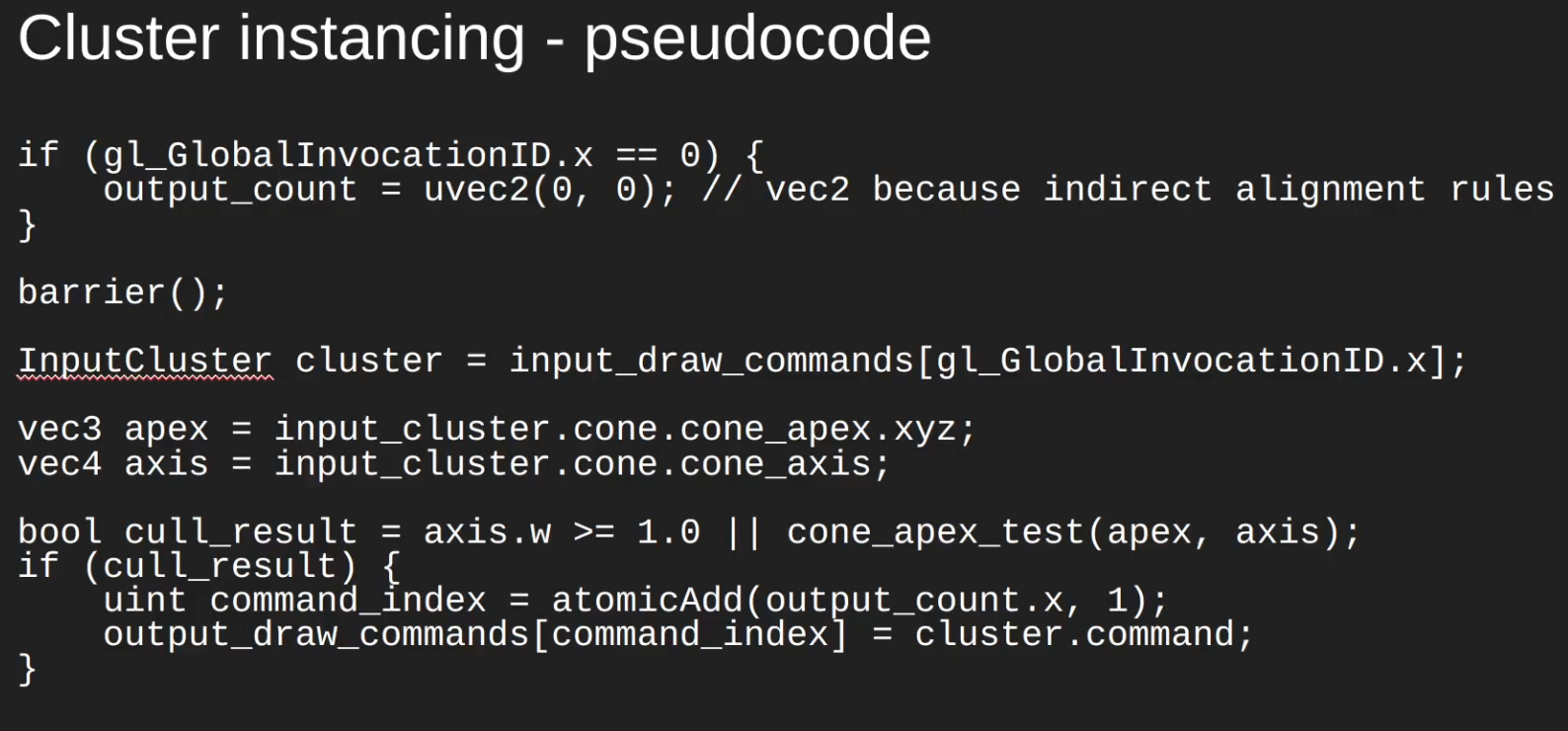 .
.
-
-
VK_HUAWEI_cluster_culling_shader.
-
MeshOptimizer
-
From what I saw in the code below, it seems to have several interesting optimizations.
-
ogldev\DemoLITION\Framework\Source\core_model.cpp:492 -
It's the last thing done when creating the mesh.
template<typename VertexType>
void CoreModel::OptimizeMesh(int MeshIndex, std::vector<uint>&Indices, std::vector<VertexType>&Vertices, std::vector<VertexType>& AllVertices)
{
    size_t NumIndices = Indices.size();
    size_t NumVertices = Vertices.size();
    // Create a remap table
    std::vector<unsigned int> remap(NumIndices);
    size_t OptVertexCount = meshopt_generateVertexRemap(remap.data(),    // dst addr
                                                        Indices.data(),  // src indices
                                                        NumIndices,      // ...and size
                                                        Vertices.data(), // src vertices
                                                        NumVertices,     // ...and size
                                                        sizeof(VertexType)); // stride
    // Allocate a local index/vertex arrays
    std::vector<uint> OptIndices;
    std::vector<VertexType> OptVertices;
    OptIndices.resize(NumIndices);
    OptVertices.resize(OptVertexCount);
    // Optimization #1: remove duplicate vertices
    meshopt_remapIndexBuffer(OptIndices.data(), Indices.data(), NumIndices, remap.data());
    meshopt_remapVertexBuffer(OptVertices.data(), Vertices.data(), NumVertices, sizeof(VertexType), remap.data());
    // Optimization #2: improve the locality of the vertices
    meshopt_optimizeVertexCache(OptIndices.data(), OptIndices.data(), NumIndices, OptVertexCount);
    // Optimization #3: reduce pixel overdraw
    meshopt_optimizeOverdraw(OptIndices.data(), OptIndices.data(), NumIndices, &(OptVertices[0].Position.x), OptVertexCount, sizeof(VertexType), 1.05f);
    // Optimization #4: optimize access to the vertex buffer
    meshopt_optimizeVertexFetch(OptVertices.data(), OptIndices.data(), NumIndices, OptVertices.data(), OptVertexCount, sizeof(VertexType));
    // Optimization #5: create a simplified version of the model
    float Threshold = 1.0f;
    size_t TargetIndexCount = (size_t)(NumIndices * Threshold);
    float TargetError = 0.0f;
    std::vector<unsigned int> SimplifiedIndices(OptIndices.size());
    size_t OptIndexCount = meshopt_simplify(SimplifiedIndices.data(), OptIndices.data(), NumIndices,
                                            &OptVertices[0].Position.x, OptVertexCount, sizeof(VertexType), TargetIndexCount, TargetError);
    static int num_indices = 0;
    num_indices += (int)NumIndices;
    static int opt_indices = 0;
    opt_indices += (int)OptIndexCount;
    printf("Num indices %d\n", num_indices);
    //printf("Target num indices %d\n", TargetIndexCount);
    printf("Optimized number of indices %d\n", opt_indices);
    SimplifiedIndices.resize(OptIndexCount);
    // Concatenate the local arrays into the class attributes arrays
    m_Indices.insert(m_Indices.end(), SimplifiedIndices.begin(), SimplifiedIndices.end());
    AllVertices.insert(AllVertices.end(), OptVertices.begin(), OptVertices.end());
    m_Meshes[MeshIndex].NumIndices = (uint)OptIndexCount;
}
Draco
-
Draco .
-
Draco is a library for compressing and decompressing 3D geometric meshes and point clouds. It is intended to improve the storage and transmission of 3D graphics.
-
By Google.
LOD, MipMap
-
Mipmap, Minification Filters, Magnification Filters .
-
MIP: Latin for 'Much In Little'.
-
It downsizes the image in powers of two.
-
-
{5:31 -> 10:10}
-
Explanation of the Filters
-
Minification:
-
Nearest, Linear, Linear_mipmap_nearest and Linear_mipmap_linear.
-
-
Magnification:
-
Nearest, Linear.
-
-
-
{10:14 -> end}
-
GLSL implementation.
-
-
{19:29 -> 21:02}
-
Differences in the Filters.
-
-
-
-
Trilinear Filtering: Linear interpolate between levels of mipmapping.
-
-
Improving the mipmap for transparent objects at a distance (foliage) - The Witness .
-
The idea is very simple: modify the content of the mipmap during its creation.
-
It shows a formula to manipulate the final result to get a better look.
-
That's all.
-
I found it interesting.
-
-
Using the full chain :
-
Advantages :
-
Hardware trilinear/anisotropic filtering benefits from having all levels available → better quality when minifying.
-
Simplifies generation: many GPU/CPU mip-generation algorithms assume a full chain.
-
No runtime fallback behavior to a coarser final level.
-
-
Disadvantages :
-
Increased memory and upload cost (sum of sizes of all mip levels).
-
Extra work to generate or upload every level (unless you generate on GPU).
-
-
-
Lower mip levels (1 < mipLevels < max) :
-
Advantages :
-
Lower memory and upload cost.
-
Useful for streaming: allocate only top K levels now, stream lower-res later.
-
Useful for textures that will rarely be minified (UI element, near camera).
-
-
Disadvantages :
-
Potentially poorer filtering when the sampler requests a lower LOD; sampling will effectively use the last available level (coarser detail).
-
If you plan to GPU-blit/generate mips, you must still have declared the target number of levels ahead of generation.
-
Some runtime tools/algorithms may assume a full chain and need adaptation.
-
-
Mesh: LOD
-
-
Godot provides a way to automatically generate less detailed meshes for LOD usage on import, then use those LOD meshes when needed automatically. This is completely transparent to the user. The meshoptimizer library is used for LOD mesh generation behind the scenes.
-
Image Formats
KTX2
-
Is a container file format for storing texture data optimized for GPU usage. It’s designed to work efficiently with modern graphics APIs like Vulkan, OpenGL, and DirectX.
Dynamic Resolution
-
 .
.
-
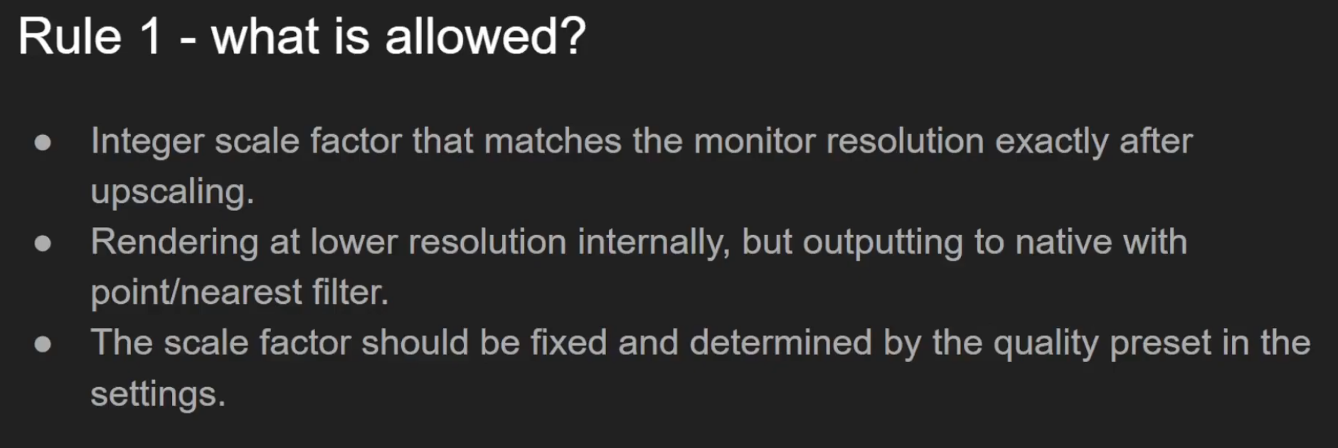 .
.
-
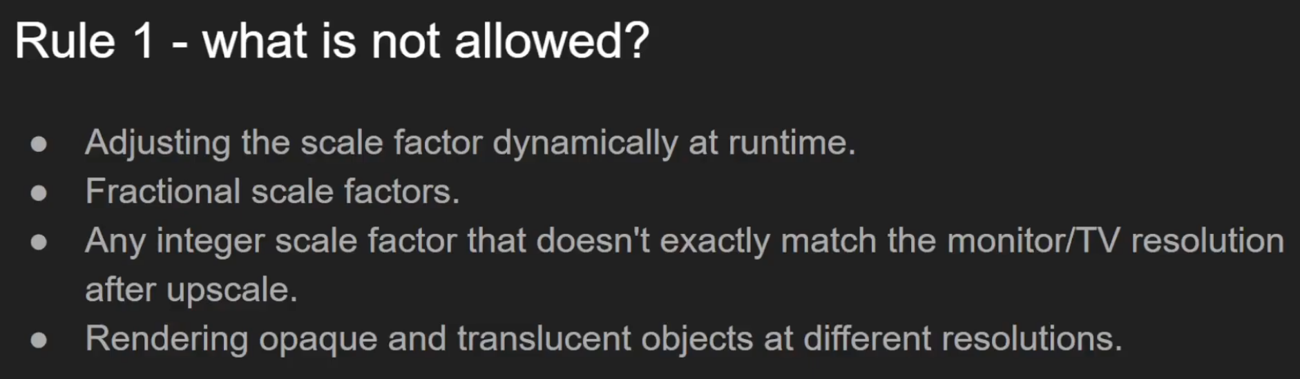 .
.
-
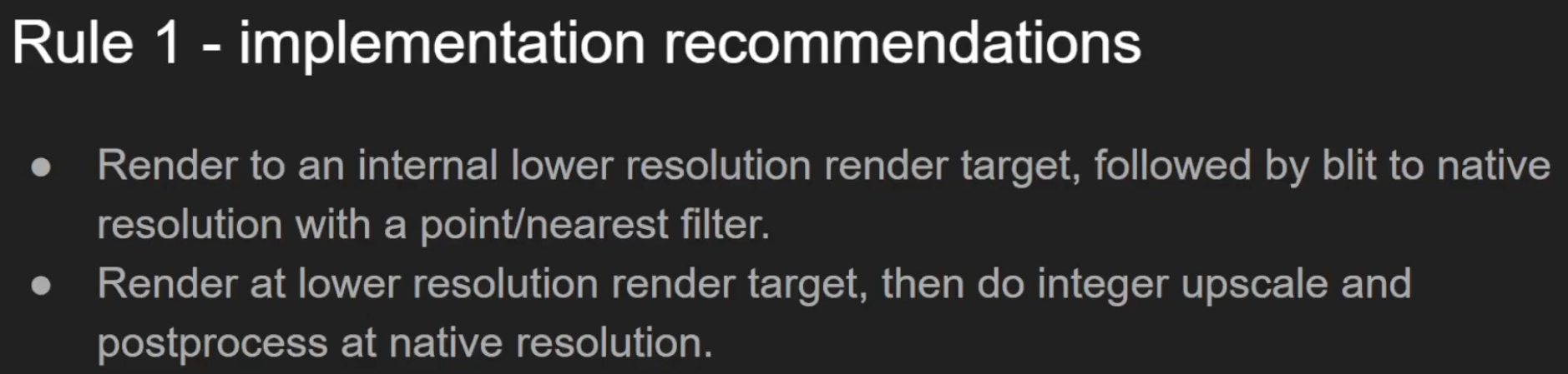 .
.
Tiling-based / VRS / Nanite
Variable Rate Shading (VRS)
-
With VRS you can specify different sampling rates for different parts of the screen. This can be used to optimize performance for either adapting the shading rate to the content, or for adapting the shading rate for things like foveated rendering in VR, where you only need full shading rate at the center of the viewport.
-
Demo .
-
VRS seems to work better with Forward than Deferred Rendering.
Tiling Post-Processing
Nanite
-
Baz - Nanite is still a deferred renderer, but I don't think Forward or Deferred Renderer is the right choice.
-
-
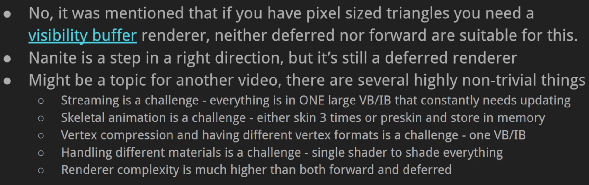 .
.
Software Based Rasterization
-
High-Performance Software Rasterization on GPUs by Laine and Karras.
-
That paper describes an all-compute rendering pipeline for the traditional 3D triangle workload. The architecture calls for sorting in the middle of the pipeline, so that in the early stage of the pipeline, triangles can be processed in arbitrary order to maximally exploit parallelism, but the output render still correctly applies the triangles in order.
-
In 3D rendering, you can almost get away with unsorted rendering, relying on Z-buffering to decide a winning fragment, but that would result in “Z-fighting” artifacts and also cause problems for semitransparent fragments.
-
Goals :
-
Our endeavor has multiple goals. First, we want to establish a firm data point of the performance of a state-of-the-art GPU software rasterizer compared to the hardware pipeline. We maintain that only a careful experiment will reveal the performance difference, as without an actual implementation there are too many unknown costs. Second, constructing a purely software-based graphics pipeline opens the opportunity to augment it with various extensions that are impossible or infeasible to fit in the hardware pipeline (without hardware modifications, that is). For example, programmable ROP calculations, trivial non-linear rasterization (e.g., [Gascuel et al. 2008]), fragment merging [Fatahalianet al. 2010], stochastic rasterization [Akenine-M¨oller et al. 2007] with decoupled sampling [Ragan-Kelley et al. 2011], etc., could be implemented as part of the programmable pipeline. Thirdly, by identifying the hot spots in our software pipeline, we hope to illuminate future hardware that would be better suited for fully programmable graphics. The complexity and versatility of the hardware graphics pipeline does not come without costs in design and testing. In an ideal situation, just a few hardware features targeted at accelerating software-based graphics would be enough to obtain decent performance, and the remaining gap would be closed by faster time-to-market and reduced design costs.
-
-
-
2D :
-
Sort-middle architecture - Raph Levien .
-
Not so easy to understand.
-
-
Fast 2D rendering - Raph Levien .
-
Not so easy to understand.
-
-