Material

Base Color / Albedo

• Diffuse albedo for non-metallic surfaces, and specular color for metallic surfaces.

• Linear RGB [0..1] .

• It should be devoid of lighting information, except for micro-occlusion.

• For Non-Metallic Materials :

  • Represents the reflected color and should be an sRGB value in the range 50-240 (strict range) or 30-240 (tolerant range).

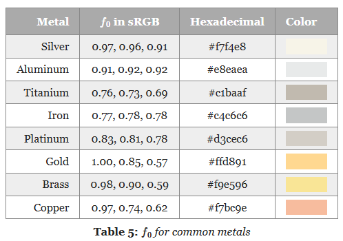
• For Metallic Materials :

  • Represents both the specular color and reflectance.

  • Use values with a luminosity of 67% to 100% (170-255 sRGB).

  • Oxidized or dirty metals should use a lower luminosity than clean metals to take into account the non-metallic components.

Roughness Value / Roughness Map

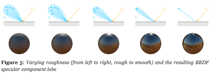
• Perceived smoothness (0.0) or roughness (1.0) of a surface. Smooth surfaces exhibit sharp reflections

• Scalar [0..1] .

• .

  • Rough (left), smooth (right).

• .

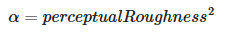
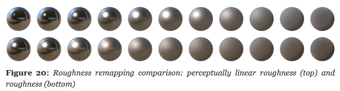
• Remapping :

  • .

  • .

Metallic Map

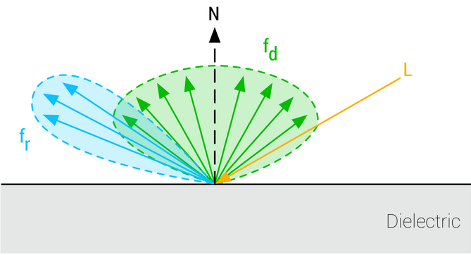
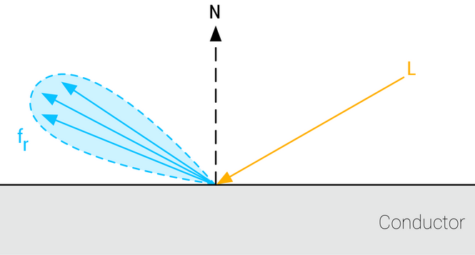
• Whether a surface appears to be dielectric (0.0) or conductor (1.0).

• Scalar [0..1] .

• Is almost a binary value. Pure conductors have a metallic value of 1 and pure dielectrics have a metallic value of 0. You should try to use values close at or close to 0 and 1. Intermediate values are meant for transitions between surface types (metal to rust for instance).

• .

  • Non-Metallic.

• .

  • Metallic.

Reflectance

Parameter

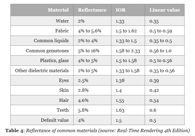
• Fresnel reflectance at normal incidence for dielectric surfaces. This replaces an explicit index of refraction

• Scalar [0..1] .

• For Non-Metallic Materials :

  • Should be set to 127 sRGB (0.5 linear, 4% reflectance) if you cannot find a proper value. Do not use values under 90 sRGB (0.35 linear, 2% reflectance).

• For Metallic Materials :

  • Is ignored (calculated from the base color).

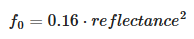
• We will use the remapping for dielectric surfaces:

  • .

  • For reflectance = 0.5 , f0 = 0.04 .

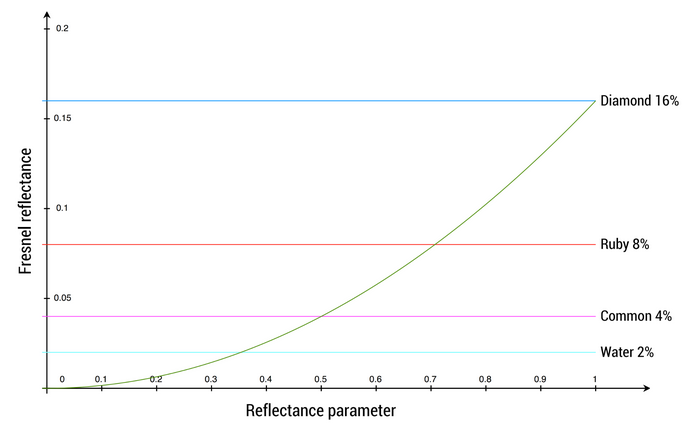
• The goal is to map onto a range that can represent the Fresnel values of both common dielectric surfaces (4% reflectance) and gemstones (8% to 16%).

• .

• The mapping function is chosen to yield a 4% Fresnel reflectance value for an input reflectance of 0.5 (or 128 on a linear RGB gray scale).

• .

  • No  real world material has a value under 2%.

• .

Emission

• Additional diffuse albedo to simulate emissive surfaces (such as neons, etc.) This parameter is mostly useful in an HDR pipeline with a bloom pass

• Linear RGB [0..1]  + exposure compensation.

Normal Map, Displacement Map

• PBR Textures in 3 minutes .

• PBR Textures Showcase .

• Bump, Normal, Displacement, and Parallax Mapping .

  • Great video. No formulas or implementation, though.

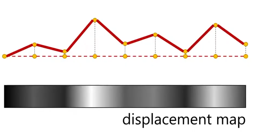
Displacement Map

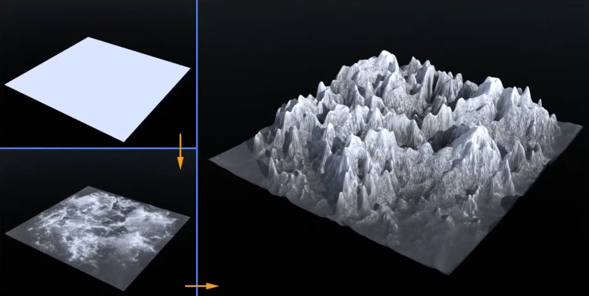
• Actually generate the geometry deformation; it's not faking anything.

• A lot more expensive then Bump Map or Normal Map.

• .

• Requirements :

  • You can have a really high-res Displacement Map, but if you don't have enough vertices to displace, then you will not get the geometric detail.

    • This is not the same for Normal Maps; a high-res Normal Map give high detail, regardless of the vertex count.

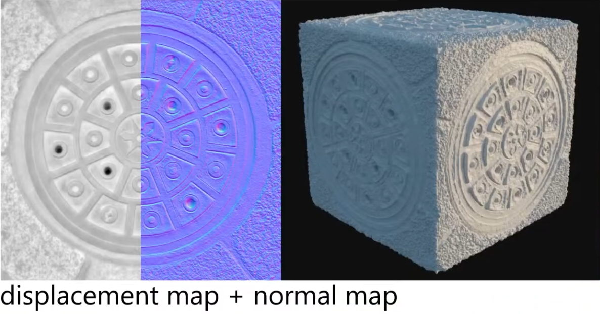
• Displacement Map vs Displacement Map + Normal Map

  • The Displacement Map is usually used with a Normal Map.

    • Just by moving vertices around, you are not  changing the normals. To see the visual changes, you need the normals that the geometry will have after the displacement.

    • How can I get the Normal Map? You can use the Displacement Map as a Bump Map, which will give you the information you need to get the Normal Map.

    • You should have a Normal Map if you intend to use the Displacement Map at runtime, as it's cheaper then having to calculate the normals on the fly.

  • .

  • You can  use a Displacement Map without a Normal Map, but you need to "apply" the Displacement Map so you calculate the new normals after the Displacement.

  • If you don't apply (and thus re-calculate the surface normals), you will need a Normal Map.

  • In the end, you need  the new normals, in one way or another.

• Used for :

  • Offline Terrain Generation.

    • .

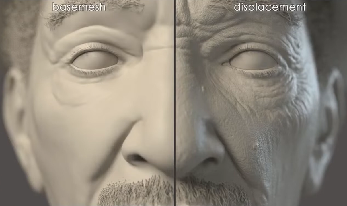
  • Offline Sculptures.

    • Some fine details that are hard to model, and you may want geometry, instead of faking with a Normal Map.

    • .

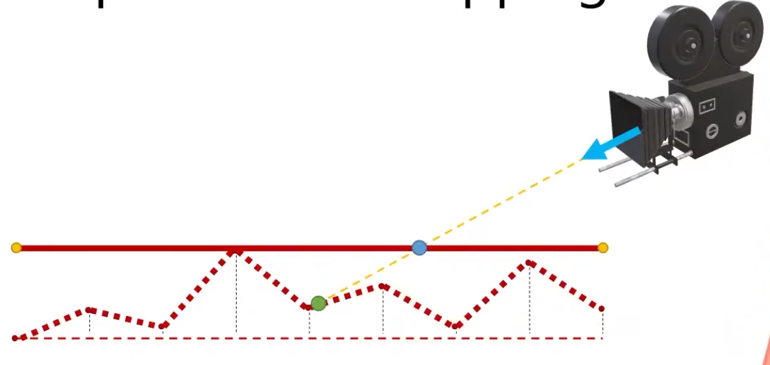
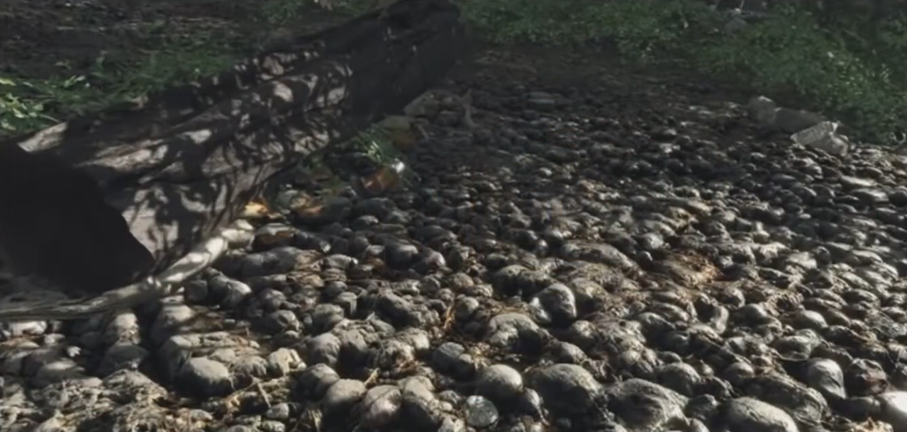
• Per-Pixel Displacement Mapping :

  • It's a technique to get the visual  of a displacement map, without generating new geometry.

  • The trick is not elevating  the geometry with the Displacement Mapping, but "craving" the geometry.

  • .

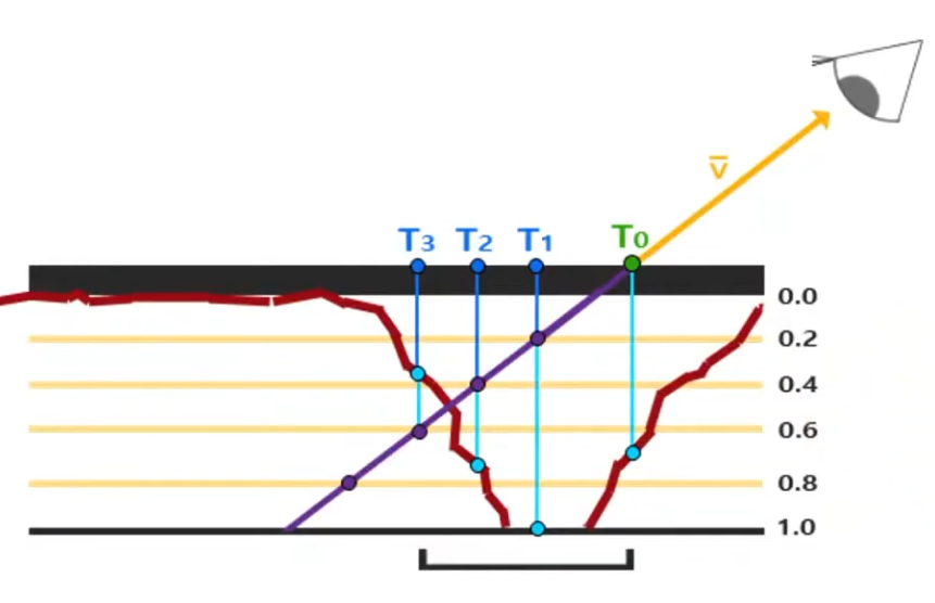
    • Renders the green point, instead of the blue point.

  • This is a lot cheaper then having a Displacement Map generating the geometry, but still has a cost, as the fragment shader needs to figure out what pixel to actually shade.

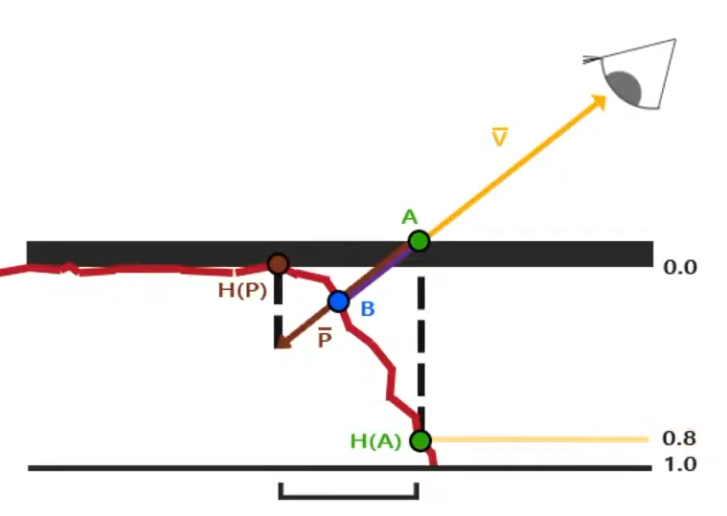
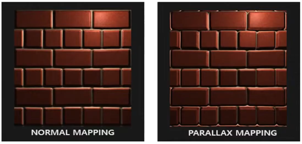
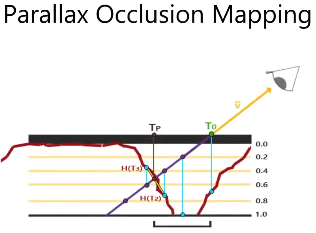
• Parallax Mapping :

  • Is a way to approximate the result of Per-Pixel Displacement Mapping .

  • .

    • With Per-Pixel Displacement Mapping , the frag shader would have to figure out what's the correct point to shade. It will look for the blue point B.

    • With Parallax Mapping , the height between the A point and the correct height H(A) is used as an approximation to determine where the blue point B is. In this example, the technique misses the B point and reaches P, but this is the final pixel that will be drawn.

      • Even tho seems like a "big miss", the final visual looks fine.

  • .

  • .

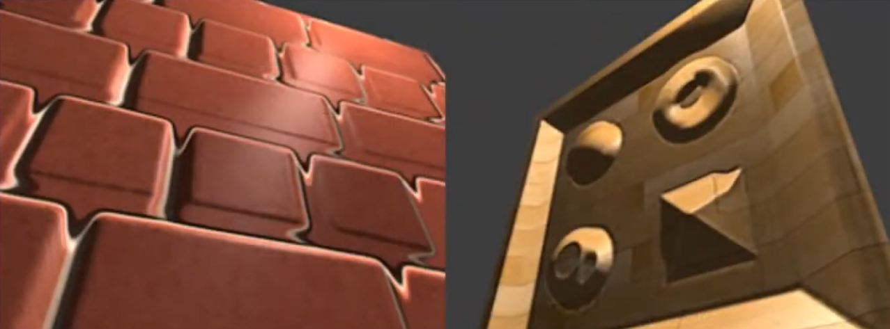
    • If the surface is rotated, things begin to not look so good.

    • Looking head on is better.

• Steep Parallax Mapping :

  • A better approximation for Per-Pixel Displacement Mapping  then Parallax Mapping , but a considerable more expensive then Parallax Mapping .

  • .

    • It does multiple texture reads instead of just one, in order to determine a better "stopping point" for the 'correct pixel to shade'.

  • .

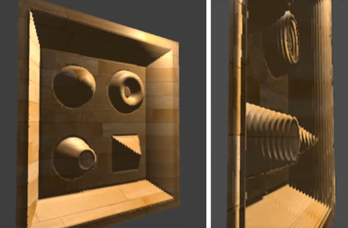
    • It's better, but if the angle is too exagerated, the problem returns.

• Parallax Occlusion Mapping :

  • A better approximation for Per-Pixel Displacement Mapping  then Step Parallax Mapping , but a bit more expensive then Step Parallax Mapping .

  • .

    • It adds one extra step at the end of the Step Parallax Mapping  evaluation.

    • This extra step doesn't perform any new texture read, it just better guesses the 'correct pixel to shade' based on the position of the previous step and the final step.

  • It gives more "continuity" for the guesses. It's smoother.

  • .

  • .

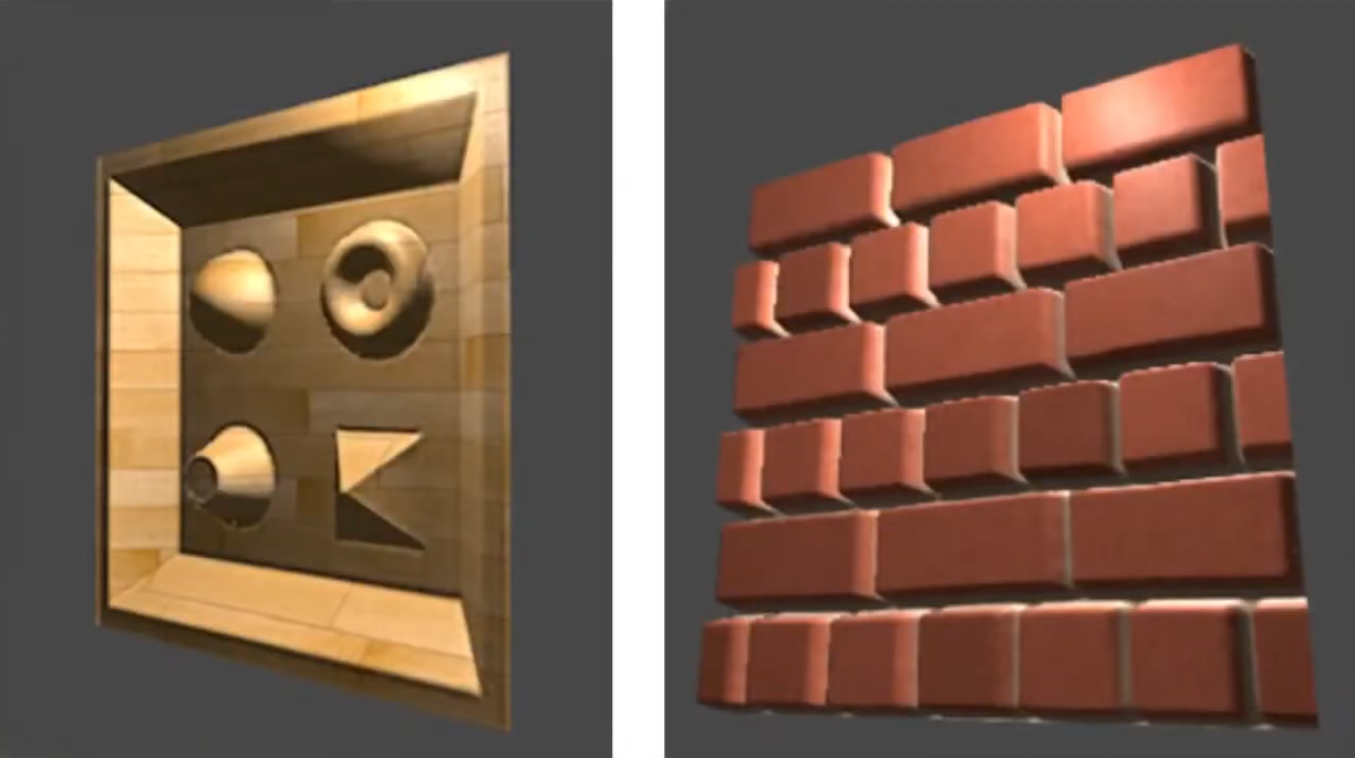
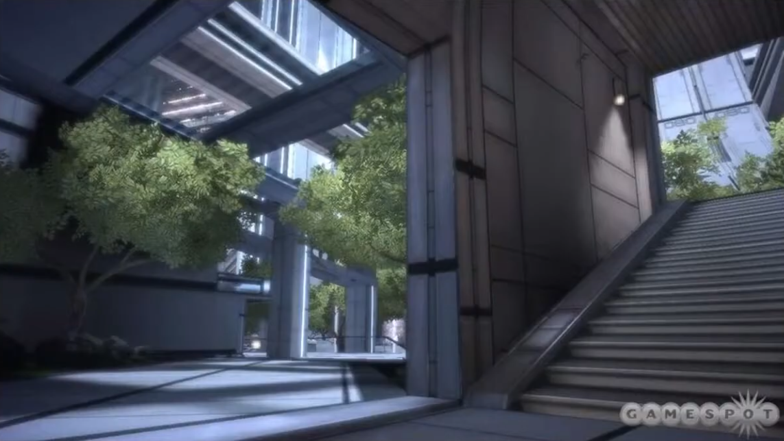
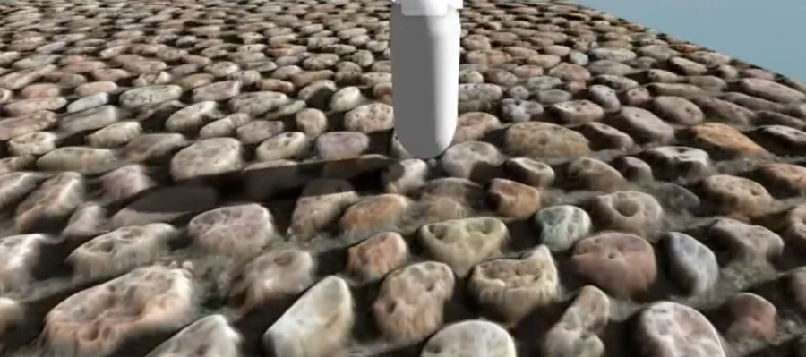
    • The stairs uses the Parallax Occlusion Mapping; it's just a flat plain.

  • .

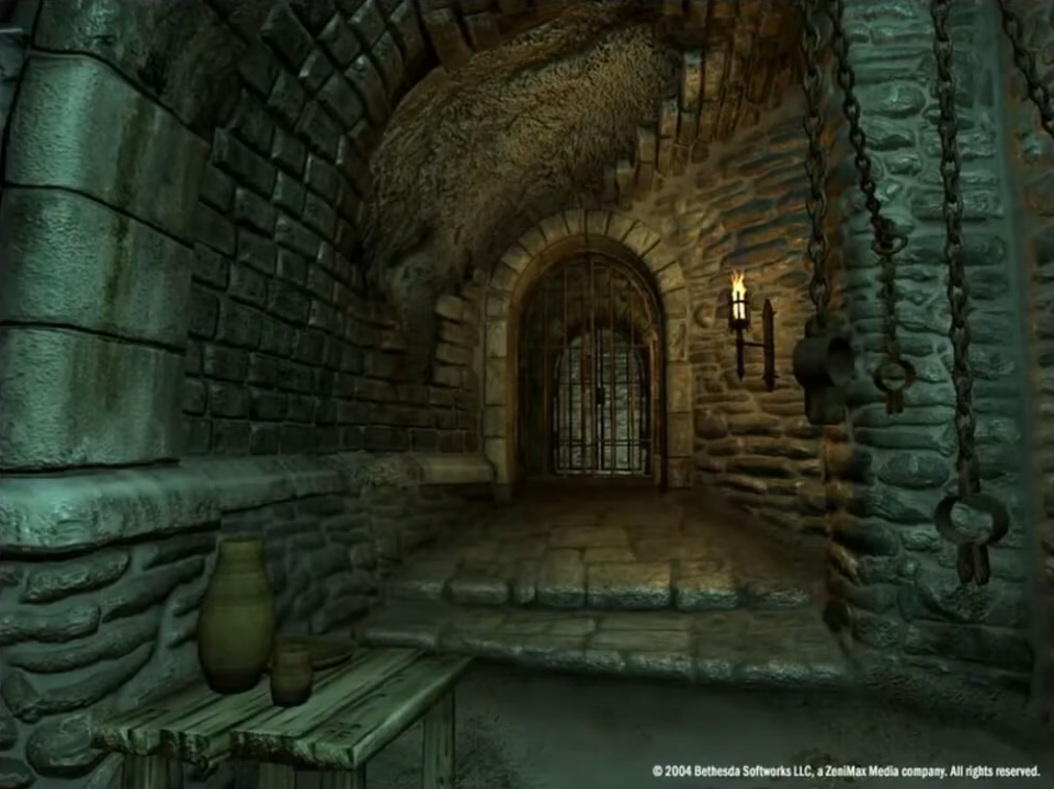
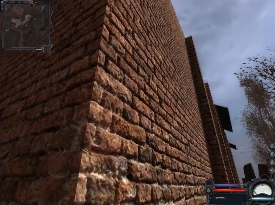
    • All the walls uses the Parallax Occlusion Mapping.

  • .

  • .

• What about shadow casting?

  • Displacement Mapping and all techniques that approximate the result of Displacement Mapping can  cast shadows.

  • .

• WebGL Demo of different displacement techniques .

  • (2025-09-12) Didn't work on Firefox, Brave, or Chrome.

Normal Map

• Tangent Space :

  • Explanation, with visualization of the Tangent Space .

  • Tech Details .

  • Tangent Space - Eric Lengyel .

    • (2025-09-15)

      • This is the one I chose to use.

      • RayLib does this same implementation in GenMeshTangents .

  • mikktspace .

    • The implementation is designed, specifically, to make the generation of tangent space as resilient as possible to a 3D model being moved from one application to another. That is generate the same tangent spaces even if there is a change in index list(s), ordering of faces/vertices of a face, and/or the removal of degenerate primitives. Both triangles and quads are supported.

    • This makes it easy for anyone to integrate the implementation into their own application and thus reproduce the same tangent spaces. This also makes the code a perfect candidate for an implementation standard. We hope the standard will be adopted by as many developers as possible.

    • The standard is used in Blender 2.57 and is also used by default in xNormal since version 3.17.5 in the form of a built-in tangent space plugin (binary and code).

  • Mikktspace in Odin .

    • Example .

• Smooth Shading / Flat Shading :

  • Apparently my procedural Meshes are smooth by default, due to my implementation.

    • If adjacent faces share the same vertex a

    • If triangles do not share vertex normals (i.e., each triangle has its own vertex normal equal to the face normal), lighting will be flat (sharp edges between faces).nd that vertex has a single normal (an average), shading will be smooth across the faces.

  • Meshes coming from models may or may not be smooth, depending on how it was imported.

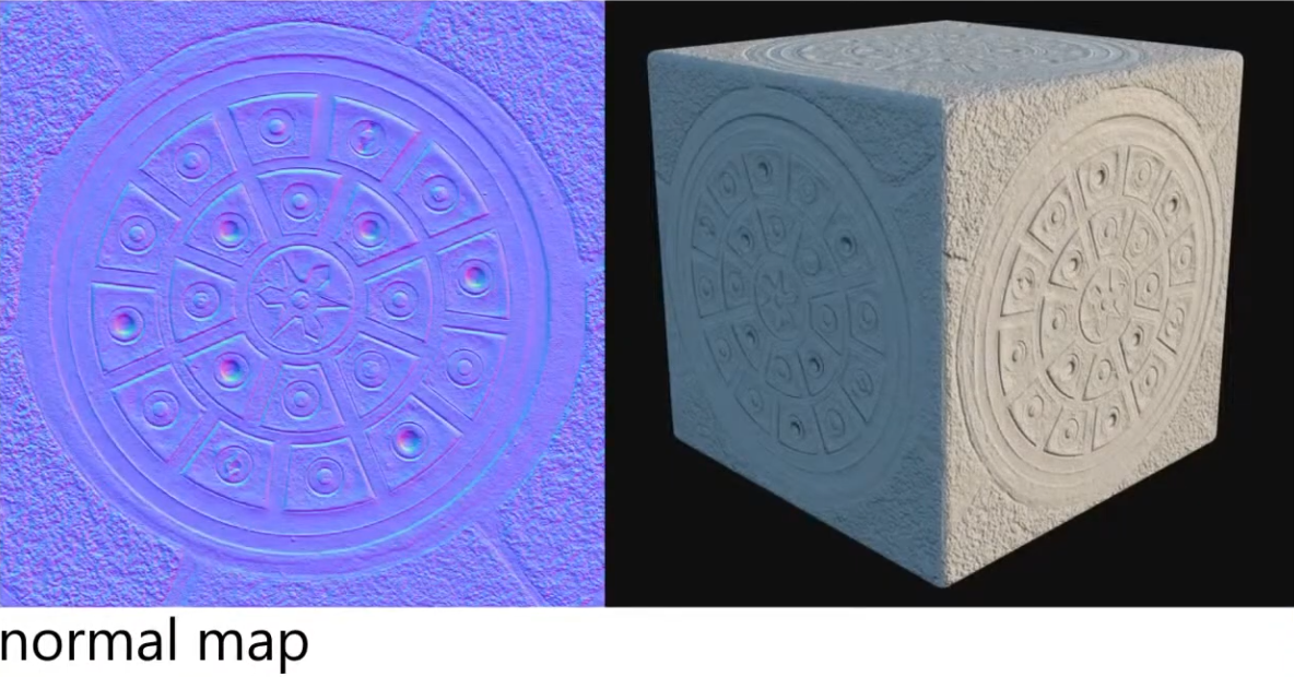
• A RGB texture encoding surface normals (X, Y, Z).

• Overrides per-pixel normal vectors, giving the illusion of complex surface detail under lighting without changing geometry.

• Used for small details/deformations; doesn't work well for something that is too deep or elevated; the illusion breaks.

• The coordinates from the Normal Map are actually in local coordinates from the point evaluated.

  • This make sense, as we want the normals to make sense, even if the character is moving.

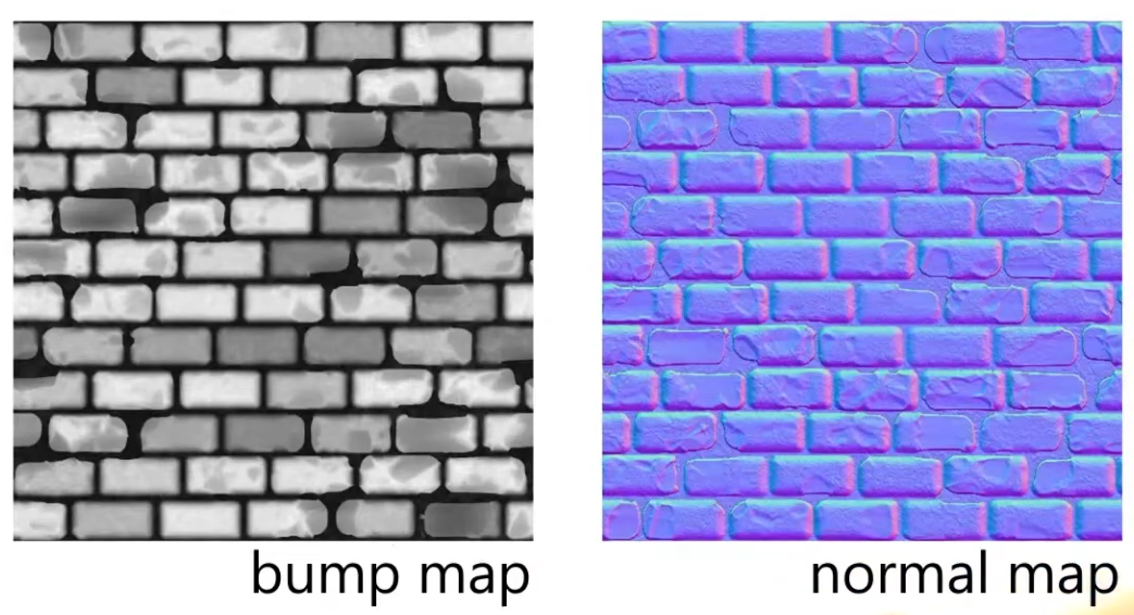
  • This is why there's a lof of blue in a normal map. The more blue the map is, the less disturbed the normal of a point is.

• Color intuition :

  • Red: inclining the normal towards the X direction (X+ == right).

  • Green: inclining towards the Y direction (Y+ == up).

  • Blue: not inclining.

• .

• NormalMap DirectX vs NormalMap OpenGL .

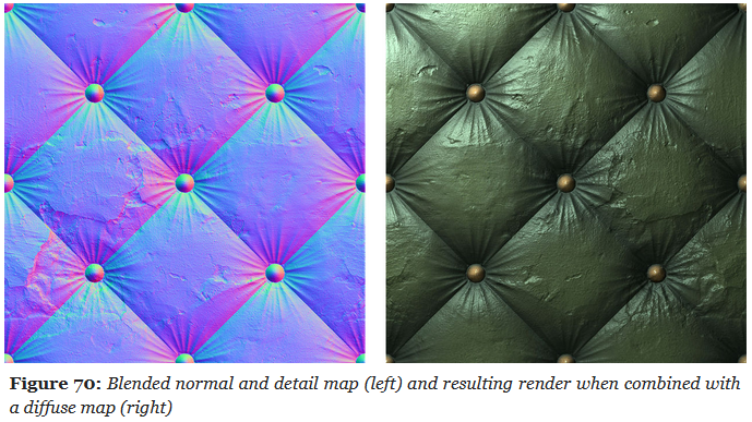
• Blending normal maps :

  • Reoriented normal mapping

  vec3 t = texture(baseMap,   uv).xyz * vec3( 2.0,  2.0, 2.0) + vec3(-1.0, -1.0,  0.0);
  vec3 u = texture(detailMap, uv).xyz * vec3(-2.0, -2.0, 2.0) + vec3( 1.0,  1.0, -1.0);
  vec3 r = normalize(t * dot(t, u) - u * t.z);
  return r;
  

  • .

  • UDN Blending :

    • Its main advantage is the low number of shader instructions it requires.

    • While it leads to a reduction in details over flat areas, UDN blending is interesting if blending must be performed at runtime.

    vec3 t = texture(baseMap,   uv).xyz * 2.0 - 1.0;
    vec3 u = texture(detailMap, uv).xyz * 2.0 - 1.0;
    vec3 r = normalize(t.xy + u.xy, t.z);
    return r;
    

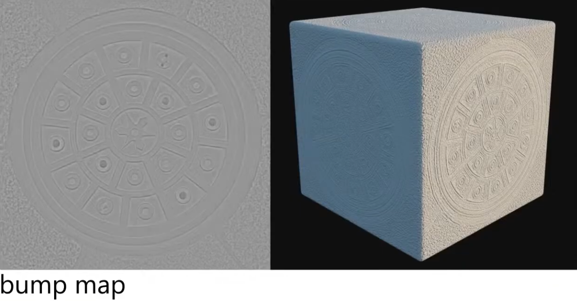
~Height Map

• Usually referred to as a Bump Map, but they aren't really  the same.

• Grayscale texture, encoding relative surface elevation; it represents the actual height/elevation values, not the variations  as a Bump Map would do.

• It can be used in different contexts:

  • To generate normals (essentially turning it into a bump/normal map).

  • To drive parallax mapping  (screen-space depth illusion).

  • To drive displacement mapping  (real geometric change).

Bump Map

• Grayscale texture where brightness represents surface height variations . White = high, black = low.

• It does not store absolute "height," but only brightness variations that are sampled to compute a local slope.

• No depth, no parallax.

• Very lightweight (single-channel grayscale).

• Typically used for adding simple surface detail in older or performance-constrained engines.

• .

• Requires additional texture reads. You have to know how the height is changing in regions around the current point.

• "Would be nice to just pre-record the normals (as that what we actually want), instead of having to compute the normals through a Bump Map? Yes! That's why a Normal Map exists".

• The Normal Map stores the normals, instead of the variation of the normals, like a Bump Map.

• .

  • Visually, at runtime, they will look exactly the same; not always, but close enough; the parameters need to be the same.

• Normal Map is the modernized version of a Bump Map.

Ambient Occlusion Map

Parameter

• Defines how much of the ambient light is accessible to a surface point. It is a per-pixel shadowing factor between 0.0 and 1.0.

• Scalar [0..1] .

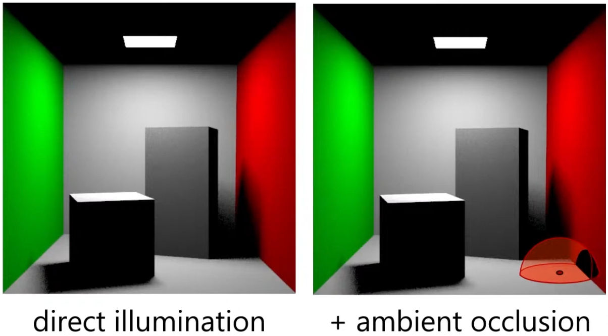
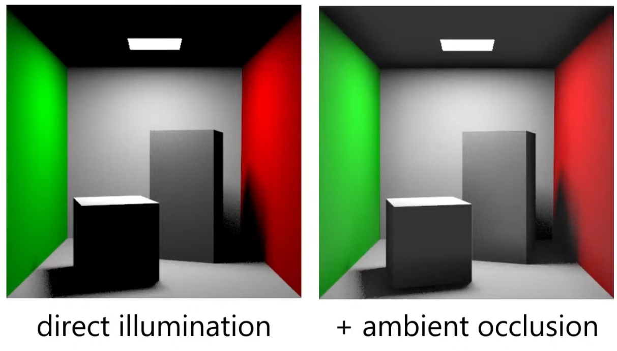
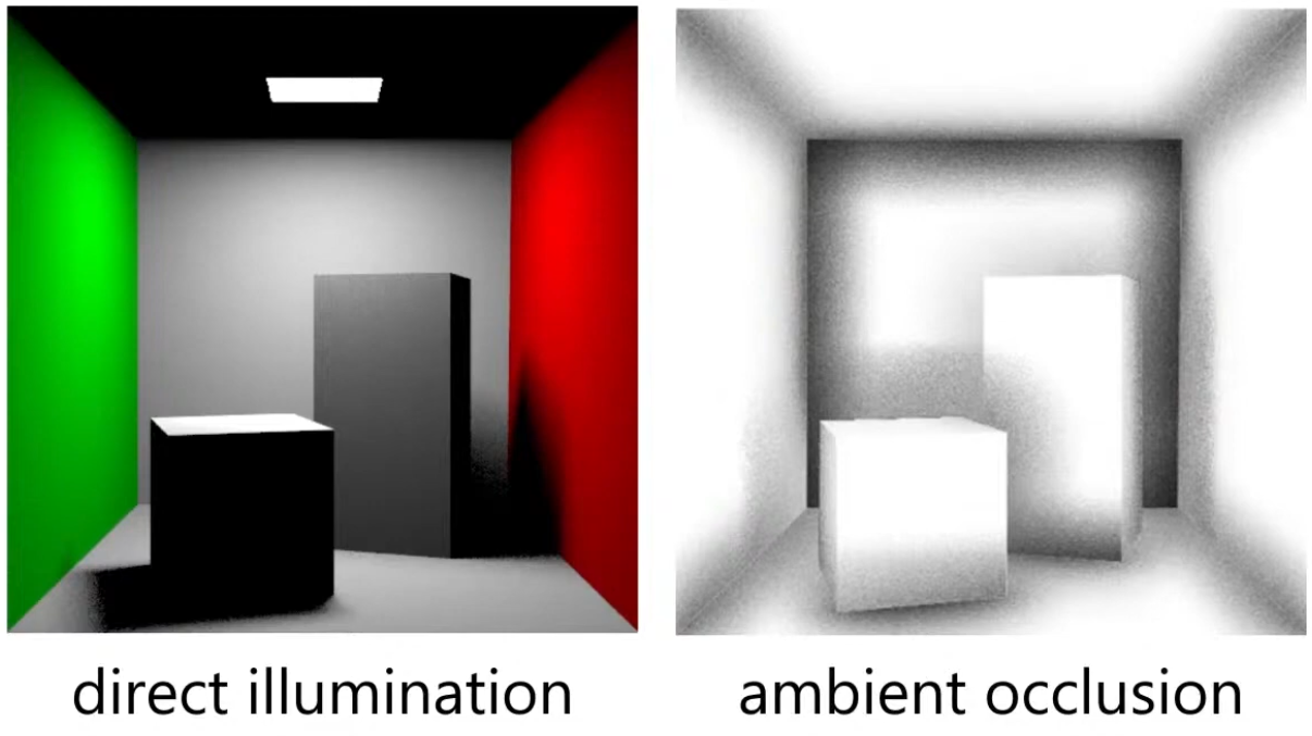
• AO is an approximation of diffuse global illumination , focusing purely on occlusion from nearby geometry, approximating how exposed each point in a scene is to ambient lighting.

• More specifically, it estimates the amount of indirect light that reaches a surface point by considering occlusion from nearby geometry.

  • Areas that are tightly enclosed or near other surfaces (e.g., corners, creases) receive less ambient light and appear darker.

  • Areas that are more open or exposed receive more ambient light and appear brighter.

• AO is not full global illumination; it ignores directional light transport and color bleeding—it’s a simplified model to capture the general “shadowing” effect of ambient light.

• The idea for Ambient Occlusion is to determine how bright or dark a region should be based on what is occluding it.

• .

• .

• .

Ambient Occlusion Map

• Diffuse :

  // diffuse indirect
  vec3 indirectDiffuse = max(irradianceSH(n), 0.0) * Fd_Lambert();
  
  // ambient occlusion
  indirectDiffuse *= texture2D(aoMap, outUV).r;
  

• Specular :

  float f90 = clamp(dot(f0, 50.0 * 0.33), 0.0, 1.0);
  // cheap luminance approximation
  float f90 = clamp(50.0 * f0.g, 0.0, 1.0);
  

  float computeSpecularAO(float NoV, float ao, float roughness) {
      return clamp(pow(NoV + ao, exp2(-16.0 * roughness - 1.0)) - 1.0 + ao, 0.0, 1.0);
  }
  
  // specular indirect
  vec3 indirectSpecular = evaluateSpecularIBL(r, perceptualRoughness);
  
  // ambient occlusion
  float ao = texture2D(aoMap, outUV).r;
  indirectSpecular *= computeSpecularAO(NoV, ao, roughness);
  

• Horizon :

  // specular indirect
  vec3 indirectSpecular = evaluateSpecularIBL(r, perceptualRoughness);
  
  // horizon occlusion with falloff, should be computed for direct specular too
  float horizon = min(1.0 + dot(r, n), 1.0);
  indirectSpecular *= horizon * horizon;
  

• Suggestions :

  • TLDR : Option 4 is the correct one, 3 is acceptable in the absence of IBL, and 1 is a non-physics-based hack.

  1. ~multiply only the albedo.

     • Blender does it this way.

     • I felt that it greatly increases the contrast in the object. Even in the most illuminated points, there are dark regions.

     • If you multiply the base color texture directly by AO (texture-level multiplication), you may inadvertently change the metallic F0 appearance. Avoid multiplying the base color used for F0 in the specular path; instead apply AO only to the diffuse/indirect parts.

  2. ~multiply only the diffuse.

     • I felt that it greatly increases the contrast in the object. Even in the most illuminated points, there are dark regions.

     • Do not multiply light_accumulation by AO — that would darken direct lighting and specular highlights.

  3. ~multiply the ambient_final

     • If you have no IBL yet, multiply the AO into ambient_final. Once you add IBL, multiply AO into the indirect diffuse term (the irradiance / ambient diffuse) and apply a reduced or rougness-weighted AO to the indirect specular if you want occlusion to affect glossy reflections.

  4. apply only to ambient indirect:

     // -> Indirect diffuse (irradiance)
     vec3 irradiance; // from diffuse irradiance probe / spherical harmonics / ambient color
     // the diffuse response (Lambertian) is usually: irradiance * albedo / PI
     vec3 ambient_diffuse = irradiance * (albedo * (1.0 / PI));
     // apply AO to indirect diffuse (AO modulates the irradiance * albedo term)
     ambient_diffuse *= ao;
     
     // ->Indirect specular (IBL)
     // prefilteredSpecular and a BRDF LUT give you the specular IBL contribution:
     vec3 prefilteredColor; // sample prefiltered environment map with roughness
     vec2 brdfLUT;          // result from split-sum integration: (scale, bias)
     vec3 ambient_specular = prefilteredColor * (brdfLUT.x * F0 + brdfLUT.y);
     // Optionally attenuate indirect specular by AO depending on roughness.
     // Rationale: very smooth surfaces reflect far-away environment less affected by local occluders.
     float specularAO = mix(1.0, ao, clamp(1.0 - roughness, 0.0, 1.0)); // lerp: smooth -> less AO effect
     ambient_specular *= specularAO;
     
     // -> Combine
     vec3 ambient_indirect = ambient_diffuse + ambient_specular;
     // final (linear)
     vec3 final_color = light_accumulation + ambient_indirect + emissive;
     return final_color;
     

Anisotropy

Parameter

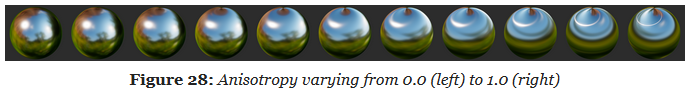
• Amount of anisotropy.

• Scalar [-1..1] .

• Note that negative values will align the anisotropy with the bitangent direction instead of the tangent direction.

• .

  • For a rough metallic surface.

Anisotropy Specular BRDF

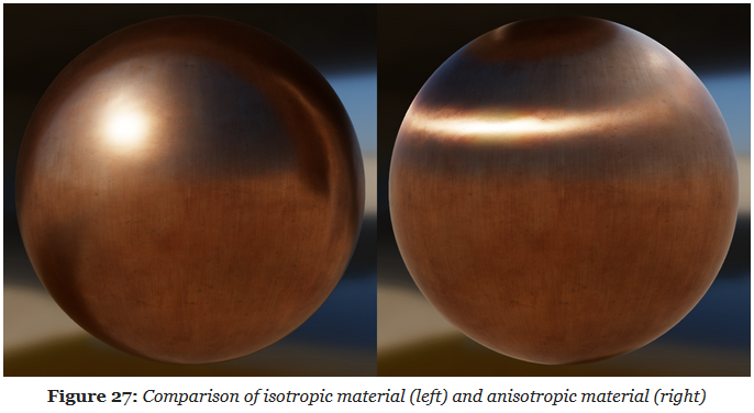
• The standard material model described previously can only describe isotropic surfaces, that is, surfaces whose properties are identical in all directions. Many real-world materials, such as brushed metal, can, however, only be replicated using an anisotropic model.

• .

• The Isotropic Specular BRDF  described previously can be modified to handle anisotropic materials.

• Burley's anisotropic NDF :

  float at = max(roughness * (1.0 + anisotropy), 0.001);
  float ab = max(roughness * (1.0 - anisotropy), 0.001);
  
  float D_GGX_Anisotropic(float NoH, const vec3 h,
          const vec3 t, const vec3 b, float at, float ab) {
      float ToH = dot(t, h);
      float BoH = dot(b, h);
      float a2 = at * ab;
      highp vec3 v = vec3(ab * ToH, at * BoH, a2 * NoH);
      highp float v2 = dot(v, v);
      float w2 = a2 / v2;
      return a2 * w2 * w2 * (1.0 / PI);
  }
  

• Anisotropic visibility function

float at = max(roughness * (1.0 + anisotropy), 0.001);
float ab = max(roughness * (1.0 - anisotropy), 0.001);

float V_SmithGGXCorrelated_Anisotropic(float at, float ab, float ToV, float BoV,
        float ToL, float BoL, float NoV, float NoL) {
    float lambdaV = NoL * length(vec3(at * ToV, ab * BoV, NoV));
    float lambdaL = NoV * length(vec3(at * ToL, ab * BoL, NoL));
    float v = 0.5 / (lambdaV + lambdaL);
    return saturateMediump(v);
}

Clear Coat

Parameter

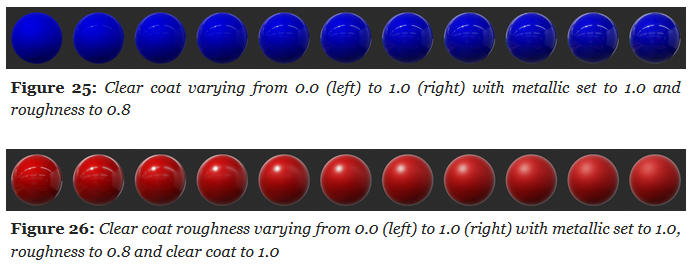
• Clear Coat :

  • Strength of the clear coat layer.

  • Scalar [0..1] .

• Clear Coat Roughness :

  • Perceived smoothness or roughness of the clear coat layer.

  • Scalar [0..1] .

• .

Clear Coat Specular BRDF

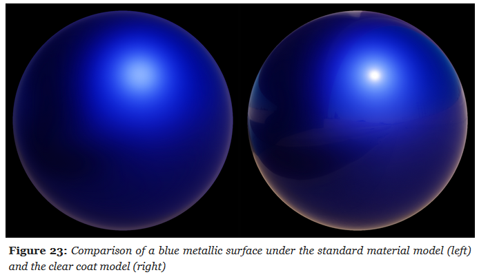
• The standard material model is a good fit for isotropic surfaces made of a single layer.

• Multi-layer materials are fairly common, particularly materials with a thin translucent layer over a standard layer.

• Examples :

  • Car paints, soda cans, lacquered wood, acrylic, etc.

• .

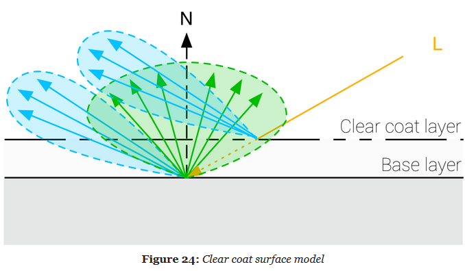
• A clear coat layer can be simulated as an extension of the standard material model by adding a second specular lobe, which implies evaluating a second specular BRDF.

• To simplify the implementation and parameterization, the clear coat layer will always be isotropic and dielectric.

• Our model will however not simulate inter reflection and refraction behaviors.

• .

• It's a Cook-Torrance  specular microfacet model, with a GGX  normal distribution function, a Kelemen  visibility function, and a Schlick Fresnel  function.

• Kelemen visibility term :

  float V_Kelemen(float LoH) {
      return 0.25 / (LoH * LoH);
  }
  

Sheen

Parameters

• Color :

  • Specular tint to create two-tone specular fabrics (defaults to 0.04 to match the standard reflectance).

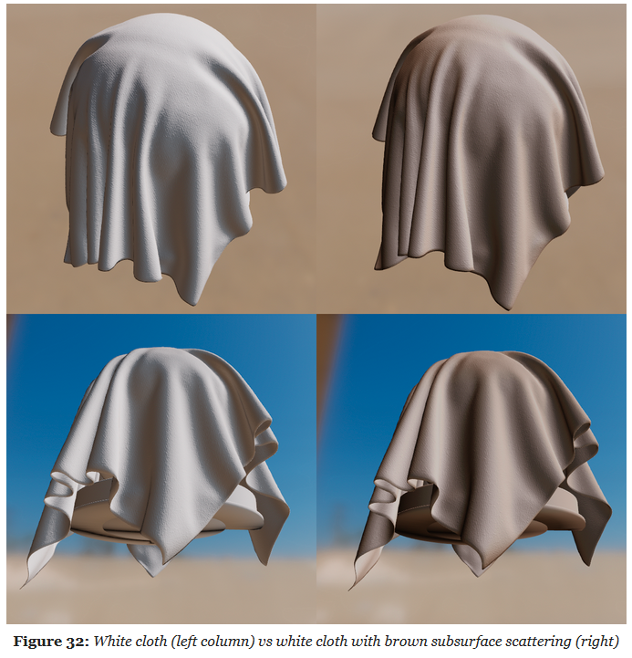
• Subsurface Color :

  • Tint for the diffuse color after scattering and absorption through the material.

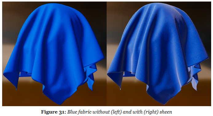
  • To create a velvet-like material, the base color can be set to black (or a dark color). Chromaticity information should instead be set on the sheen color. To create more common fabrics such as denim, cotton, etc. use the base color for chromaticity and use the default sheen color or set the sheen color to the luminance of the base color.

Cloth Specular BRDF

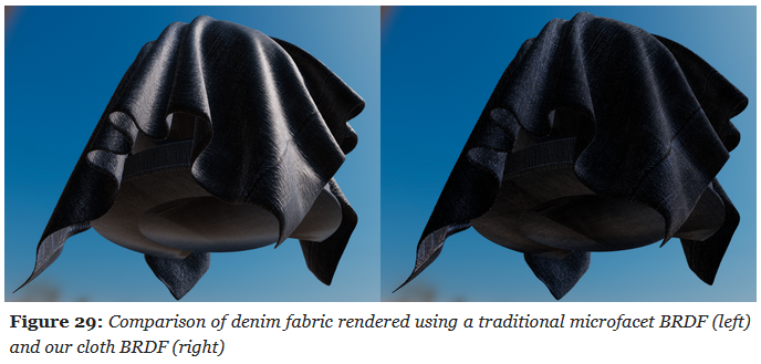
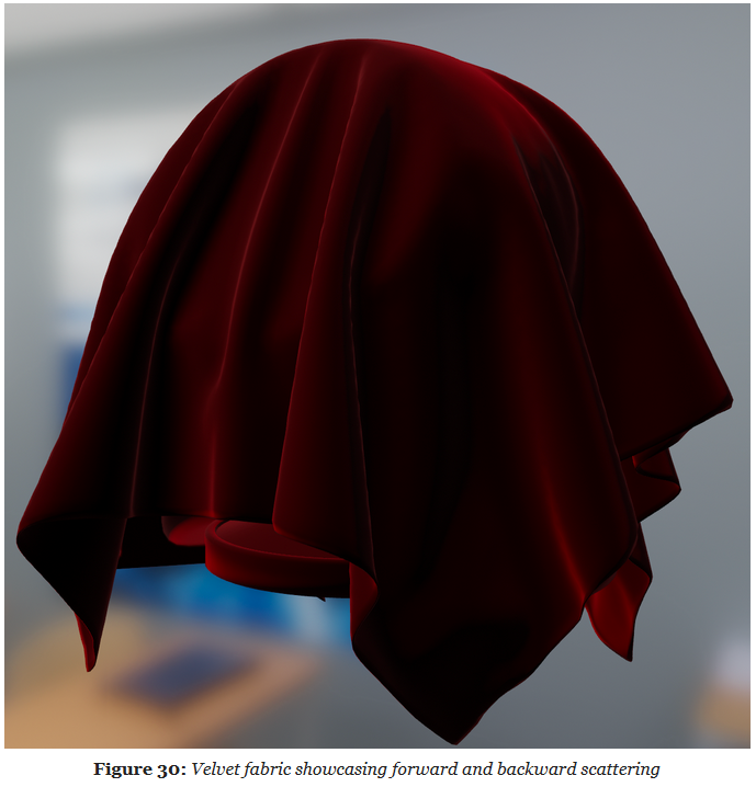
• All the material models described previously are designed to simulate dense surfaces, both at a macro and at a micro level. Clothes and fabrics are however often made of loosely connected threads that absorb and scatter incident light. The microfacet BRDFs presented earlier do a poor job of recreating the nature of cloth due to their underlying assumption that a surface is made of random grooves that behave as perfect mirrors. When compared to hard surfaces, cloth is characterized by a softer specular lobe with a large falloff and the presence of fuzz lighting, caused by forward/backward scattering. Some fabrics also exhibit two-tone specular colors (velvets for instance).

• A traditional microfacet BRDF fails to capture the appearance of a sample of denim fabric. The surface appears rigid (almost plastic-like), more similar to a tarp than a piece of clothing. This figure also shows how important the softer specular lobe caused by absorption and scattering is to the faithful recreation of the fabric.

• .

• Velvet is an interesting use case for a cloth material model. As shown below, this type of fabric exhibits strong rim lighting due to forward and backward scattering. These scattering events are caused by fibers standing straight at the surface of the fabric. When the incident light comes from the direction opposite to the view direction, the fibers will forward-scatter the light. Similarly, when the incident light from the same direction as the view direction, the fibers will scatter the light backward.

• .

• The cloth specular BRDF  we use is a modified microfacet BRDF as described by Ashikhmin  and Premoze .

• Ashikhmin's Velvet NDF :

  float D_Ashikhmin(float roughness, float NoH) {
      // Ashikhmin 2007, "Distribution-based BRDFs"
      float a2 = roughness * roughness;
      float cos2h = NoH * NoH;
      float sin2h = max(1.0 - cos2h, 0.0078125); // 2^(-14/2), so sin2h^2 > 0 in fp16
      float sin4h = sin2h * sin2h;
      float cot2 = -cos2h / (a2 * sin2h);
      return 1.0 / (PI * (4.0 * a2 + 1.0) * sin4h) * (4.0 * exp(cot2) + sin4h);
  }
  

• Charlie NDF :

  • Optimized to properly fit in half float formats.

  float D_Charlie(float roughness, float NoH) {
      // Estevez and Kulla 2017, "Production Friendly Microfacet Sheen BRDF"
      float invAlpha  = 1.0 / roughness;
      float cos2h = NoH * NoH;
      float sin2h = max(1.0 - cos2h, 0.0078125); // 2^(-14/2), so sin2h^2 > 0 in fp16
      return (2.0 + invAlpha) * pow(sin2h, invAlpha * 0.5) / (2.0 * PI);
  }
  

Cloth Diffuse BRDF

• Sheen :

  • To offer better control over the appearance of cloth and to give users the ability to recreate two-tone specular materials, we introduce the ability to directly modify the specular reflectance.

  • .

• Subsurface Scattering :

  • .