-
 .
.
-
From the Real-Time Rendering 4th Edition.
-
-
 .
.
-
By Ola Olsson.
-
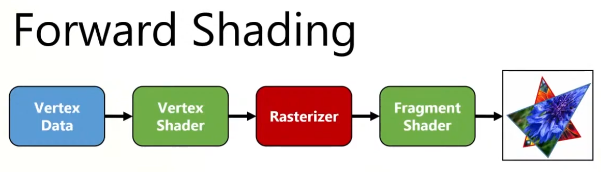
Forward Rendering
Forward
-
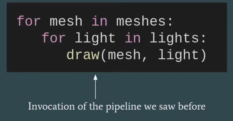
Geometry is shaded as it is drawn. For each triangle/pixel, the fragment shader loops over the lights that affect that object (or uses some per-object light set).
-
Lighting for a fragment is computed when that fragment is shaded, using the set of lights you feed to that draw call/shader.
-
Shading and output to the final render target happen in one pass.
-
 .
.
-
Overdraw happens, as the back triangle is shaded , but the front triangle overwrites the color on the screen.
-
-
 .
.
-
"Multipass forward rendering".
-
-
 .
.
-
 .
.
Tiled Forward Shading
-
Tiled shading can be applied to both forward and deferred rendering methods.
-
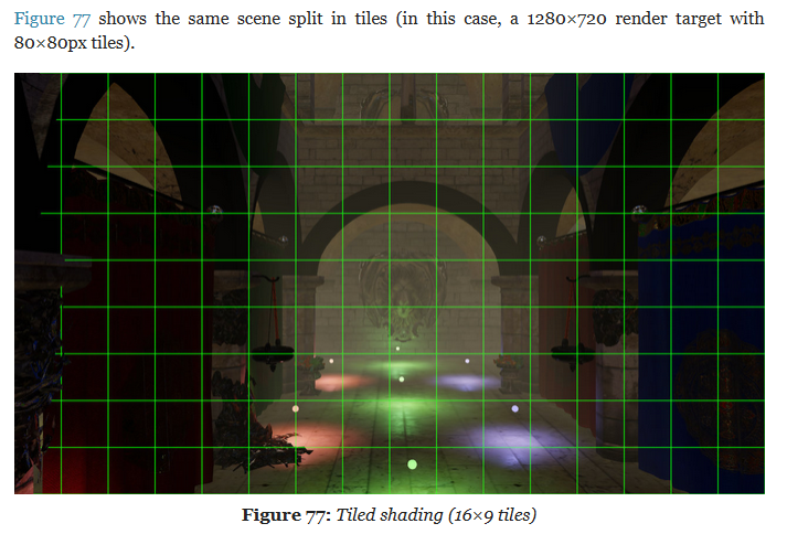
The idea is to split the screen into a grid of tiles and, for each tile, find the list of lights that affect the pixels within that tile.
-
This has the advantage of reducing overdraw (in deferred rendering) and shading computations of large objects (in forward rendering).
-
However, this technique suffers from depth discontinuity issues that can lead to large amounts of extraneous work.
Gathering the lights
-
We now need to access all relevant lights for each pixel sequentially.
-
Just using a global list of lights is, of course, terribly inefficient.
-
On the other hand, creating lists of lights for each pixel individually is both slow and requires lots of storage.
-
Tiled shading strikes a balance, where we create lists for tiles of pixels.
-
The list must be conservative, storing all lights that may affect any sample within the tile.
-
So we trade some compute performance for bandwidth, which, as we have seen, is a good tradeoff on modern GPUs.
-
Each tile contains a single list of all the lights that might influence any of the pixels inside.
-
This list is shared between the pixels, so overhead for list maintenance and fetching is low.
Constructing the list
-
 .
.
-
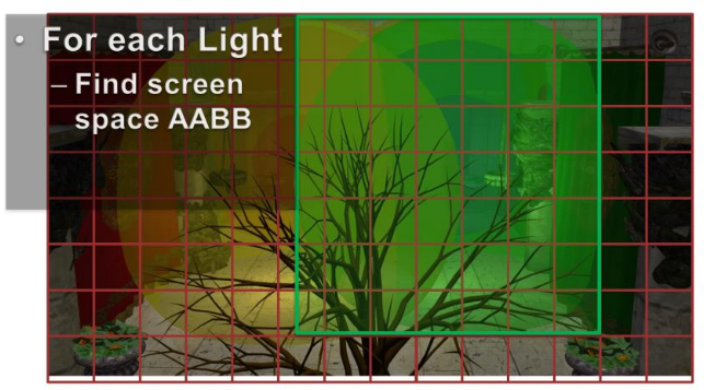
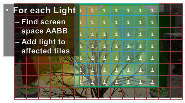
For each light, establish the screen space bounding box, illustrated for the green light.
-
Then add the index of the light to all overlapped tiles.
-
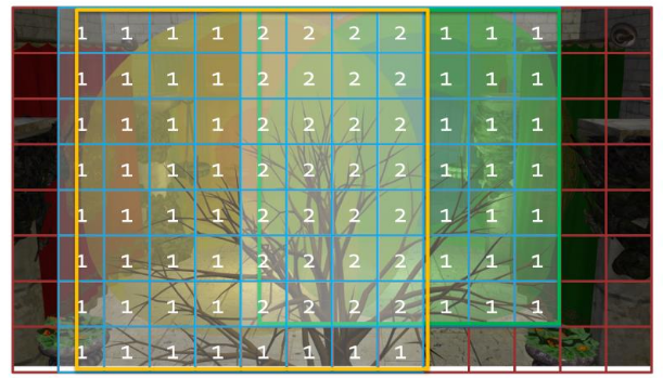
Then repeat this process for all remaining lights.
-
The illustration only shows the counts, so you need to imagine the lists being built as well.
-
In practice, we’d also do a conservative per-tile min/max depth test to cull away lights occupying empty space.
Vertex Shader
-
Vertex Output:
struct VertexShaderOutput { float3 positionVS : TEXCOORD0; // View space position. float2 texCoord : TEXCOORD1; // Texture coordinate float3 tangentVS : TANGENT; // View space tangent. float3 binormalVS : BINORMAL; // View space binormal. float3 normalVS : NORMAL; // View space normal. float4 position : SV_POSITION; // Clip space position. };-
I chose to do all of the lighting in view space, as opposed to world space, because it is easier to work in view space coordinates when implementing deferred shading and forward+ rendering techniques.
-
The
SV_POSITIONsemantic is applied to the output value from the vertex shader to specify that the value is used as the clip space position, but this semantic can also be applied to an input variable of a pixel shader. WhenSV_POSITIONis used as an input semantic to a pixel shader, the value is the position of the pixel in screen space. In both the deferred shading and the forward+ shaders, I will use this semantic to get the screen space position of the current pixel.
VertexShaderOutput VS_main( AppData IN ) { VertexShaderOutput OUT; OUT.position = mul( ModelViewProjection, float4( IN.position, 1.0f ) ); OUT.positionVS = mul( ModelView, float4( IN.position, 1.0f ) ).xyz; OUT.tangentVS = mul( ( float3x3 )ModelView, IN.tangent ); OUT.binormalVS = mul( ( float3x3 )ModelView, IN.binormal ); OUT.normalVS = mul( ( float3x3 )ModelView, IN.normal ); OUT.texCoord = IN.texCoord; return OUT; }-
You will notice that I am pre-multiplying the input vectors by the matrices. This indicates that the matrices are stored in column-major order by default.
-
Fragment Shader Inputs
-
Material :
-
Since some material properties can also have an associated texture (for example, diffuse textures, specular textures, or normal textures), we will also use the material to indicate if those textures are present on the object.
struct Material { float4 GlobalAmbient; //-------------------------- ( 16 bytes ) float4 AmbientColor; //-------------------------- ( 16 bytes ) float4 EmissiveColor; //-------------------------- ( 16 bytes ) float4 DiffuseColor; //-------------------------- ( 16 bytes ) float4 SpecularColor; //-------------------------- ( 16 bytes ) // Reflective value. float4 Reflectance; //-------------------------- ( 16 bytes ) float Opacity; float SpecularPower; // For transparent materials, IOR > 0. float IndexOfRefraction; bool HasAmbientTexture; //-------------------------- ( 16 bytes ) bool HasEmissiveTexture; bool HasDiffuseTexture; bool HasSpecularTexture; bool HasSpecularPowerTexture; //-------------------------- ( 16 bytes ) bool HasNormalTexture; bool HasBumpTexture; bool HasOpacityTexture; float BumpIntensity; //-------------------------- ( 16 bytes ) float SpecularScale; float AlphaThreshold; float2 Padding; //--------------------------- ( 16 bytes ) }; //--------------------------- ( 16 * 10 = 160 bytes )-
GlobalAmbient-
Describes the ambient contribution applied to all objects in the scene globally. Technically, this variable should be a global variable (not specific to a single object), but since there is only a single material at a time in the pixel shader, it’s fine to put it here.
-
-
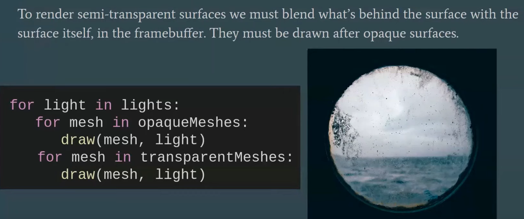
Opacity-
Determines the total opacity of an object. This value can make objects appear transparent. This property is used to render semi-transparent objects in the transparent pass. If the opacity value is less than one (1 being fully opaque and 0 being fully transparent), the object is considered transparent and rendered in the transparent pass instead of the opaque pass.
-
-
SpecularPower-
Determines how shiny the object appears.
-
-
IndexOfRefraction-
Can be applied to objects that should refract light through them. Since refraction requires environment mapping techniques not implemented in this experiment, this variable will not be used here.
-
-
BumpIntensity-
If a model has a bump map, the material’s
HasBumpTextureproperty is set totrueand the model is bump-mapped instead of normal-mapped. -
Normal and bump maps are mutually exclusive, so they can reuse the same texture slot assignment.
-
-
SpecularScale-
Scales the specular power value read from a specular power texture. Since textures usually store values as unsigned normalized values, when sampling from the texture the value is read as a floating-point value in the range of
[0..1]. A specular power of 1.0 doesn’t make much sense, so the specular power value read from the texture will be scaled bySpecularScalebefore being used for the final lighting computation.
-
-
AlphaThreshold-
Can be used to discard pixels whose opacity is below a certain value using the “discard” command in the pixel shader. This is useful for “cut-out” materials where the object does not need alpha blending but should have holes (for example, a chain-link fence).
-
-
-
The material properties are passed to the pixel shader using a constant buffer.
cbuffer Material : register( b2 ) { Material Mat; }; Texture2D AmbientTexture : register( t0 ); Texture2D EmissiveTexture : register( t1 ); Texture2D DiffuseTexture : register( t2 ); Texture2D SpecularTexture : register( t3 ); Texture2D SpecularPowerTexture : register( t4 ); Texture2D NormalTexture : register( t5 ); Texture2D BumpTexture : register( t6 ); Texture2D OpacityTexture : register( t7 ); -
Lights :
StructuredBuffer<uint> LightIndexList: register( t9 ); Texture2D<uint2> LightGrid: register( t10 ); struct Light { /** * Position for point and spot lights (World space). */ float4 PositionWS; //--------------------------------------------------------------( 16 bytes ) /** * Direction for spot and directional lights (World space). */ float4 DirectionWS; //--------------------------------------------------------------( 16 bytes ) /** * Position for point and spot lights (View space). */ float4 PositionVS; //--------------------------------------------------------------( 16 bytes ) /** * Direction for spot and directional lights (View space). */ float4 DirectionVS; //--------------------------------------------------------------( 16 bytes ) /** * Color of the light. Diffuse and specular colors are not separated. */ float4 Color; //--------------------------------------------------------------( 16 bytes ) /** * The half angle of the spotlight cone. */ float SpotlightAngle; /** * The range of the light. */ float Range; /** * The intensity of the light. */ float Intensity; /** * Disable or enable the light. */ bool Enabled; //--------------------------------------------------------------( 16 bytes ) /** * Is the light selected in the editor? */ bool Selected; /** * The type of the light. */ uint Type; float2 Padding; //--------------------------------------------------------------( 16 bytes ) //--------------------------------------------------------------( 16 * 7 = 112 bytes ) };-
SpotlightAngle-
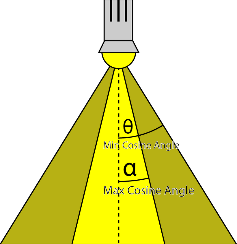
Is the half-angle of the spotlight cone expressed in degrees. Working in degrees is more intuitive than in radians. The spotlight angle is converted to radians in the shader when computing the cosine of the angle between the spotlight direction and the light vector.
-
-
Range-
For point lights, the range is the radius of the sphere that represents the light; for spotlights, it’s the length of the cone that represents the light. Directional lights don’t use range because they are considered infinitely far away, pointing in the same direction everywhere.
-
-
Intensity-
Modulates the computed light contribution. By default, this value is 1 but can make some lights brighter or dimmer than others.
-
-
Enabled-
Lights with
Enabledset tofalseare skipped in the shader.
-
-
Selected-
When a light is selected in the scene, its visual representation appears darker (less transparent) to indicate selection.
-
-
Type-
Can have one of the following values:
#define POINT_LIGHT 0 #define SPOT_LIGHT 1 #define DIRECTIONAL_LIGHT 2 -
-
Spot lights, point lights and directional lights are not separated into different structs and all of the properties necessary to define any of those light types are stored in a single struct.
-
The Position variable only applies to point and spot lights while the Direction variable only applies to spot and directional lights.
-
I store both world space and view space position and direction vectors because I find it easier to work in world space in the application then convert the world space vectors to view space before uploading the lights array to the GPU.
-
This way I do not need to maintain multiple light lists at the cost of additional space that is required on the GPU. But even 10,000 lights only require 1.12 MB on the GPU so I figured this was a reasonable sacrifice. But minimizing the size of the light structs could have a positive impact on caching on the GPU and improve rendering performance.
-
I chose not to separate the diffuse and specular color contributions because it is rare that these values differ.
-
The lights array is accessed through a StructuredBuffer . Most lighting shader implementations will use a constant buffer to store the lights array but constant buffers are limited to 64 KB in size which means that it would be limited to about 570 lights before running out of constant memory on the GPU. Structured buffers are stored in texture memory which is limited to the amount of texture memory available on the GPU (usually in the GB range on desktop GPUs). Texture memory is also very fast on most GPUs so storing the lights in a structured buffer did not impose a performance impact. In fact, on my particular GPU (NVIDIA GeForce GTX 680) I noticed a considerable performance improvement when I moved the lights array to a structure buffer.
StructuredBuffer<Light> Lights : register( t8 );
-
Fragment Shader
float3 ExpandNormal( float3 n )
{
    return n * 2.0f - 1.0f;
}

float4 DoNormalMapping( float3x3 TBN, Texture2D tex, sampler s, float2 uv )
{
    float3 normal = tex.Sample( s, uv ).xyz;
    normal = ExpandNormal( normal );

    // Transform normal from tangent space to view space.
    normal = mul( normal, TBN );
    return normalize( float4( normal, 0 ) );
}

float4 DoBumpMapping( float3x3 TBN, Texture2D tex, sampler s, float2 uv, float bumpScale )
{
    // Sample the heightmap at the current texture coordinate.
    float height = tex.Sample( s, uv ).r * bumpScale;
    // Sample the heightmap in the U texture coordinate direction.
    float heightU = tex.Sample( s, uv, int2( 1, 0 ) ).r * bumpScale;
    // Sample the heightmap in the V texture coordinate direction.
    float heightV = tex.Sample( s, uv, int2( 0, 1 ) ).r * bumpScale;

    float3 p = { 0, 0, height };
    float3 pU = { 1, 0, heightU };
    float3 pV = { 0, 1, heightV };

    // normal = tangent x bitangent
    float3 normal = cross( normalize(pU - p), normalize(pV - p) );

    // Transform normal from tangent space to view space.
    normal = mul( normal, TBN );

    return float4( normal, 0 );
}

float4 DoDiffuse( Light light, float4 L, float4 N )
{
    float NdotL = max( dot( N, L ), 0 );
    return light.Color * NdotL;
}

float4 DoSpecular( Light light, Material material, float4 V, float4 L, float4 N )
{
    float4 R = normalize( reflect( -L, N ) );
    float RdotV = max( dot( R, V ), 0 );

    return light.Color * pow( RdotV, material.SpecularPower );
}

// Compute the attenuation based on the range of the light.
float DoAttenuation( Light light, float d )
{
    return 1.0f - smoothstep( light.Range * 0.75f, light.Range, d );
}

LightingResult DoPointLight( Light light, Material mat, float4 V, float4 P, float4 N )
{
    LightingResult result;

    float4 L = light.PositionVS - P;
    float distance = length( L );
    L = L / distance;

    float attenuation = DoAttenuation( light, distance );

    result.Diffuse = DoDiffuse( light, L, N ) *
                      attenuation * light.Intensity;
    result.Specular = DoSpecular( light, mat, V, L, N ) *
                       attenuation * light.Intensity;

    return result;
}


float DoSpotCone( Light light, float4 L )
{
    // If the cosine angle of the light's direction
    // vector and the vector from the light source to the point being
    // shaded is less than minCos, then the spotlight contribution will be 0.
    float minCos = cos( radians( light.SpotlightAngle ) );
    // If the cosine angle of the light's direction vector
    // and the vector from the light source to the point being shaded
    // is greater than maxCos, then the spotlight contribution will be 1.
    float maxCos = lerp( minCos, 1, 0.5f );
    float cosAngle = dot( light.DirectionVS, -L );
    // Blend between the minimum and maximum cosine angles.
    return smoothstep( minCos, maxCos, cosAngle );
}

LightingResult DoSpotLight( Light light, Material mat, float4 V, float4 P, float4 N )
{
    LightingResult result;

    float4 L = light.PositionVS - P;
    float distance = length( L );
    L = L / distance;

    float attenuation = DoAttenuation( light, distance );
    float spotIntensity = DoSpotCone( light, L );

    result.Diffuse = DoDiffuse( light, L, N ) *
                       attenuation * spotIntensity * light.Intensity;
    result.Specular = DoSpecular( light, mat, V, L, N ) *
                       attenuation * spotIntensity * light.Intensity;

    return result;
}

LightingResult DoDirectionalLight( Light light, Material mat, float4 V, float4 P, float4 N )
{
    LightingResult result;

    float4 L = normalize( -light.DirectionVS );

    result.Diffuse = DoDiffuse( light, L, N ) * light.Intensity;
    result.Specular = DoSpecular( light, mat, V, L, N ) * light.Intensity;

    return result;
}


// This lighting result is returned by the
// lighting functions for each light type.
struct LightingResult
{
    float4 Diffuse;
    float4 Specular;
};

LightingResult DoLighting( StructuredBuffer<Light> lights, Material mat, float4 eyePos, float4 P, float4 N )
{
    float4 V = normalize( eyePos - P );

    LightingResult totalResult = (LightingResult)0;

    for ( int i = 0; i < NUM_LIGHTS; ++i )
    {
        LightingResult result = (LightingResult)0;

        // Skip lights that are not enabled.
        if ( !lights[i].Enabled ) continue;
        // Skip point and spot lights that are out of range of the point being shaded.
        if ( lights[i].Type != DIRECTIONAL_LIGHT &&
             length( lights[i].PositionVS - P ) > lights[i].Range ) continue;

        switch ( lights[i].Type )
        {
        case DIRECTIONAL_LIGHT:
        {
            result = DoDirectionalLight( lights[i], mat, V, P, N );
        }
        break;
        case POINT_LIGHT:
        {
            result = DoPointLight( lights[i], mat, V, P, N );
        }
        break;
        case SPOT_LIGHT:
        {
            result = DoSpotLight( lights[i], mat, V, P, N );
        }
        break;
        }
        totalResult.Diffuse += result.Diffuse;
        totalResult.Specular += result.Specular;
    }

    return totalResult;
}


[earlydepthstencil]
float4 PS_main( VertexShaderOutput IN ) : SV_TARGET
{
    // Everything is in view space.
    float4 eyePos = { 0, 0, 0, 1 };
    Material mat = Mat;

    // Diffuse
    float4 diffuse = mat.DiffuseColor;
    if ( mat.HasDiffuseTexture )
    {
        float4 diffuseTex = DiffuseTexture.Sample( LinearRepeatSampler, IN.texCoord );
        if ( any( diffuse.rgb ) )
        {
            diffuse *= diffuseTex;
        }
        else
        {
            diffuse = diffuseTex;
        }
    }

    // Opacity
    float alpha = diffuse.a;
    if ( mat.HasOpacityTexture )
    {
        // If the material has an opacity texture, use that to override the diffuse alpha.
        alpha = OpacityTexture.Sample( LinearRepeatSampler, IN.texCoord ).r;
    }

    // Ambient
    float4 ambient = mat.AmbientColor;
    if ( mat.HasAmbientTexture )
    {
        float4 ambientTex = AmbientTexture.Sample( LinearRepeatSampler, IN.texCoord );
        if ( any( ambient.rgb ) )
        {
            ambient *= ambientTex;
        }
        else
        {
            ambient = ambientTex;
        }
    }
    // Combine the global ambient term.
    ambient *= mat.GlobalAmbient;

    // Emissive
    float4 emissive = mat.EmissiveColor;
    if ( mat.HasEmissiveTexture )
    {
        float4 emissiveTex = EmissiveTexture.Sample( LinearRepeatSampler, IN.texCoord );
        if ( any( emissive.rgb ) )
        {
            emissive *= emissiveTex;
        }
        else
        {
            emissive = emissiveTex;
        }
    }

    // Specular
    if ( mat.HasSpecularPowerTexture )
    {
        mat.SpecularPower = SpecularPowerTexture.Sample( LinearRepeatSampler, IN.texCoord ).r \
                            * mat.SpecularScale;
    }

    // Normal mapping
    if ( mat.HasNormalTexture )
    {
        // For scenes with normal mapping, I don't have to invert the binormal.
        float3x3 TBN = float3x3( normalize( IN.tangentVS ),
                                 normalize( IN.binormalVS ),
                                 normalize( IN.normalVS ) );

        N = DoNormalMapping( TBN, NormalTexture, LinearRepeatSampler, IN.texCoord );
    }
    // Bump mapping
    else if ( mat.HasBumpTexture )
    {
        // For most scenes using bump mapping, I have to invert the binormal.
        float3x3 TBN = float3x3( normalize( IN.tangentVS ),
                                 normalize( -IN.binormalVS ),
                                 normalize( IN.normalVS ) );

        N = DoBumpMapping( TBN, BumpTexture, LinearRepeatSampler, IN.texCoord, mat.BumpIntensity );
    }
    // Just use the normal from the model.
    else
    {
        N = normalize( float4( IN.normalVS, 0 ) );
    }

    float4 P = float4( IN.positionVS, 1 );


    LightingResult lit = DoLighting( Lights, mat, eyePos, P, N );

    diffuse *= float4( lit.Diffuse.rgb, 1.0f ); // Discard the alpha value from the lighting calculations.

    float4 specular = 0;
    if ( mat.SpecularPower > 1.0f ) // If specular power is too low, don't use it.
    {
        specular = mat.SpecularColor;
        if ( mat.HasSpecularTexture )
        {
            float4 specularTex = SpecularTexture.Sample( LinearRepeatSampler, IN.texCoord );
            if ( any( specular.rgb ) )
            {
                specular *= specularTex;
            }
            else
            {
                specular = specularTex;
            }
        }
        specular *= lit.Specular;
    }

    // Get the index of the current pixel in the light grid.
    uint2 tileIndex = uint2( floor(IN.position.xy / BLOCK_SIZE) );

    // Get the start position and offset of the light in the light index list.
    uint startOffset = LightGrid[tileIndex].x;
    uint lightCount = LightGrid[tileIndex].y;

    LightingResult lit = (LightingResult)0; // DoLighting( Lights, mat, eyePos, P, N );

    for ( uint i = 0; i < lightCount; i++ )
    {
        uint lightIndex = LightIndexList[startOffset + i];
        Light light = Lights[lightIndex];

        LightingResult result = (LightingResult)0;

        switch ( light.Type )
        {
        case DIRECTIONAL_LIGHT:
        {
            result = DoDirectionalLight( light, mat, V, P, N );
        }
        break;
        case POINT_LIGHT:
        {
            result = DoPointLight( light, mat, V, P, N );
        }
        break;
        case SPOT_LIGHT:
        {
            result = DoSpotLight( light, mat, V, P, N );
        }
        break;
        }
        lit.Diffuse += result.Diffuse;
        lit.Specular += result.Specular;
    }

    diffuse *= float4( lit.Diffuse.rgb, 1.0f ); // Discard the alpha value from the lighting calculations.
    specular *= lit.Specular;

    return float4( ( ambient + emissive + diffuse + specular ).rgb, alpha * mat.Opacity );
}
-
EarlyDepthStencil :
-
The
[earlydepthstencil]attribute before the function indicates that the GPU should take advantage of early depth and stencil culling. This causes the depth/stencil tests to be performed before the pixel shader is executed. This attribute cannot be used on shaders that modify the pixel’s depth value by outputting a value using theSV_Depthsemantic. Since this pixel shader only outputs a color value using theSV_TARGETsemantic, it can take advantage of early depth/stencil testing to provide a performance improvement when a pixel is rejected. Most GPUs will perform early depth/stencil tests anyway even without this attribute, and adding this attribute to the pixel shader did not have a noticeable impact on performance, but I decided to keep the attribute anyway. -
Since all lighting computations are performed in view space, the eye position (the camera position) is always (0, 0, 0).
-
This is a nice side effect of working in view space: the camera’s eye position does not need to be passed as an additional parameter to the shader.
-
Cool.
-
-
-
First, we need to gather the material properties. If the material has textures associated with its various components, the textures will be sampled before the lighting is computed. After the material properties have been initialized, all the lights in the scene will be iterated, and the lighting contributions will be accumulated and modulated with the material properties to produce the final pixel color.
-
Comments :
-
Diffuse :
-
The
anyHLSL intrinsic function can be used to determine if any of the color components are non-zero. -
If the material also has a diffuse texture associated with it, then the color from the diffuse texture will be blended with the material’s diffuse color. If the material’s diffuse color is black (0, 0, 0, 0), then the material’s diffuse color will simply be replaced by the color in the diffuse texture.
-
-
Opacity :
-
By default, the fragment’s transparency value is determined by the alpha component of the diffuse color. If the material has an opacity texture associated with it, the red component of the opacity texture is used as the alpha value, overriding the alpha value in the diffuse texture. In most cases, opacity textures store only a single channel in the first component of the color returned from the Sample method. To read from a single-channel texture, we must read from the red channel, not the alpha channel. The alpha channel of a single-channel texture will always be 1, so reading the alpha channel from the opacity map (which is most likely a single-channel texture) would not provide the required value.
-
-
-
Lighting :
-
The lighting calculations for the forward rendering technique are performed in the
DoLightingfunction. This function accepts the following arguments:-
lights: The lights array (as a structured buffer) -
mat: The material properties that were just computed -
eyePos: The position of the camera in view space (which is always (0, 0, 0)) -
P: The position of the point being shaded in view space -
N: The normal of the point being shaded in view space
-
-
The view vector (
V) is computed from the eye position and the position of the shaded pixel in view space. -
 .
.
-
etc
-
Wicked Engine :
-
All the lights inside the camera are binned to small 8×8 pixel tiles on the screen. Each tile will thus have a minimal list of lights that should be iterated by every pixel inside when lighting up the surface.
-
The main optimizations I’ve used for some years now is the “2.5D culling” and the “flat bit arrays” methods, which I really liked.
-
I rearranged the light loops so they always operate strictly on one light type (directional/point/spot), which gave some minor performance improvement. So instead of one big loop that checks the type of light and calls the appropriate function, now there are 3 loops for each type. This also allowed to avoid all the tile checking for directional lights, because they are always affecting the full screen, that specific loop is just going over all of them which simplifies the shader further.
-
Visibility Buffer :
-
The main twist to the forward rendering is the inclusion of a secondary “visibility buffer”, to aid with effects that would better fit into a deferred renderer.
-
I always wanted to support all the post processing that deferred rendering supports, but normally forward rendering doesn’t write any G-Buffer textures to allow this. Some years ago I used a thin G-buffer for this written by the depth prepass.
-
Now the depth-prepass for the main camera writes a UINT texture that contains primitive IDs, this is called the visibility buffer.
-
This is some overhead compared to depth-only pass, but less than writing a G-buffer with multiple textures.
-
From this primitiveID texture any shader can get per-pixel information about any surface properties: depth, normal, roughness, velocity, etc.
-
The nice thing about it that we can get this on the async compute queue too, and that’s exactly what happens.
-
After the visibility buffer is completed in the prepass, the graphics queue continues rendering shadow maps, planar reflections and updating environment probes, while the compute queue starts working independently on rendering a G-buffer from the visibility buffer, but only if some effects are turned on that would require this:
-
depth buffer: it is always created from the visibility buffer. The normal depth buffer is always kept in depth write state, it’s never used as a sampled texture. This way the depth test efficiency remains the highest for the color and transparent passes later.
-
velocity: if any of the following effects are turned on: Temporal AA, Motion Blur, FSR upscaling, ray traced shadows/reflections/diffuse, SSR…
-
normal, roughness: if any of the following effects are turned on: SSR, ray traced reflections
-
some other params are simply retrieved from visibility buffer just on demand if effects need it, but not saved as a texture: for example face normal
-
light buffers: these are not separated, so things like blurred diffuse subsurface scattering is not supported. I support a simple wrapped and tinted NdotL term for subsurface scattering instead.
-
-
What does this texture actually store? It’s a single channel 32-bit UINT texture, and normally that wouldn’t be enough to store both primitive and instance ID. But there is a workaround, in which I store 25 bits of meshlet ID and 7 bits of primitive ID. A regular mesh wouldn’t fit into it, since it limits to 128 triangles, but with a lookup table it’s possible to manage.
-
-
Disadvantages
-
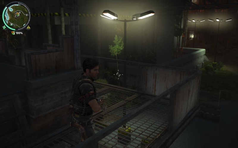
Tiled shading groups samples in rectangular screen-space tiles, using the min and max depth within each tile to define sub frustums. Thus, tiles which contain depth values that are close together, e.g. from a single surface, will be represented with small bounding volumes. However, for tiles where one or more depth discontinuities occur, the depth bounds of the tile must encompass all the empty space between the sample groups (illustrated in Figure 1). This reduces light culling efficiency, in the worst case degenerating to a pure 2D test. This results in a strong dependency between view and performance, which highly is undesirable in real-time applications, as it becomes difficult to guarantee consistent rendering performance at all times.
-
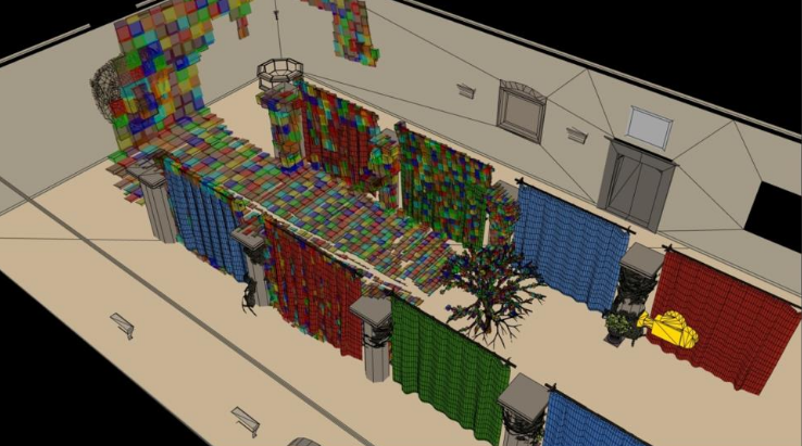
Visually, this means:
-
 .
.
-
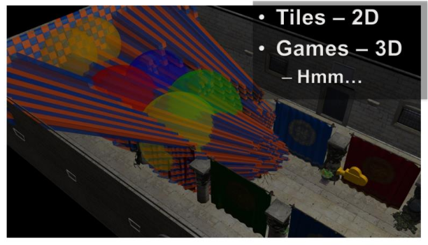
Toggling on the light geometry, we see that there is a lot of overlap, even in the empty space behind the tree.
-
We now should be able to start seeing the shape of the problem with 2D tiles in a 3D world.
-
 .
.
-
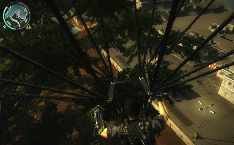
In 3D:
-
 .
.
-
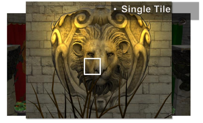
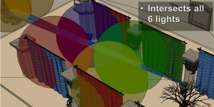
While actually some of the samples, from the tree, are affected zero of these lights. While the tiger in the wall would only need two of the lights.
-
There is a fairly fundamental problem with tiled shading. The basic problem stems from that we are making the intersection between lights and geometry samples, both of which are 3D entities, in a 2D screen space.
-
The main practical issue with this is that the resulting light assignment is highly view dependent. This means that we cannot author scenes with any strong guarantee on performance, as a given view of the scene may have a significantly higher screen space light density than average.
-
For example, we’d like to be able to construct a scene with, say, maximum 4 lights affecting any part of the scene. In this case, we would like shading cost to be proportional to this, and stable, given different view points.
-
Unfortunately, no such correlation exists for tiled shading. In other words shading times are unpredictable, which is a major problem for a real time application.
-
Avalanche Studios :
-
The two tiled solutions need quite a bit of massaging to work reasonable well in all situations, especially with large amounts of depth discontinuities. There are proposed solutions that mitigate the problem, such as 2.5D culling, but they further complicate the code.
-
I didn’t have to go look for a problematic area, in fact, it was right there in front of my face. This shows how common these scenes actually are in real games, and certainly so in the games that we make.
-
 .
.
-
We are still using a deferred engine, but we could change to forward at any time should we decide that to be better. The important part is, however, that the transparency passes can now use the same lighting structure as the deferred passes, making it a unified lighting solution.
-
-
Samples
-
Forward, Deferred, Tile Forward Shading - DirectX11, HLSL - Sample - Jeremiah van Oosten 2024 .
-
There are 30,000,000,000 files, etc, C++, Visual Studio, CMake, etc. Jeebs.
-
The only relevant things are the shaders:
-
GraphicsTest\Assets\shaders\CommonInclude.hlsl -
GraphicsTest\Assets\shaders\ForwardPlusRendering.hlsl.
-
-
Papers and Presentations
-
Forward+: Bringing Deferred Lighting to the Next Level - AMD 2012 .
-
Forward, Deferred, Tiled Forward - Jeremiah Van Oosten - 2015 .
-
C++, shaders in HLSL.
-
There's a sample above.
-
-
Demo .
-
Demo .
-
Tiled Forward Shading vs Tiled Deferred Rendering - AMD 2013 (Jason Stewart and Gareth Thomas).-
The presentation is somewhat poor and the graphics are questionable.
-
No real-world lighting cases are presented.
-
"Have you looked into Forward Clustered?" Yea, but have not implemented, they are hours worth of work. I don't know if the extra complexity is worth, but I'll probably test it at some point.
-
They use Virtual Point Lights for GI, which sounds suspicious.
-
"Extensions to the Tiled Forward"
-
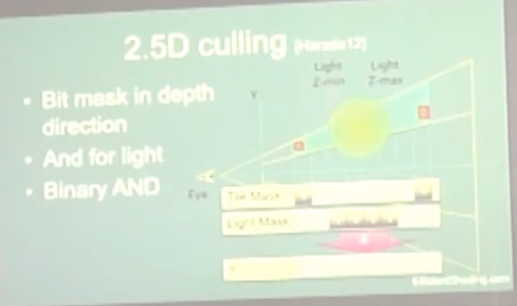
2.5D Culling :
-
2.5D Light Culling for Tiled Forward - Wicked Engine 2017 .
-
Depth discontinuity is the enemy of Forward+.
-
With a more aggressive culling we can eliminate false positives and have a much faster render.
-
-
 .
.
-
Avalanche Studios :
-
Criticizes the use of 2.5D Culling, considering that Cluster Shading yields a better result with less effort.
-
This is explained and demonstrated on pages 112 to 121 of this presentation: Efficient Real-Time Shading with Many Lights - Ola Olsson, Emil Persson (Avalanche) - 2014 .
-
2.5D Culling.
-
-
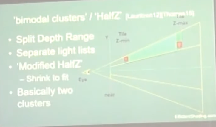
Bimodal Clusters / HalfZ :
-
 .
.
-
-
Ola Olsson:
-
This extensions have the problems of:
-
Lack of generality: slopes / multiple layers.
-
No solution for transparency.
-
Require depth pre-pass, as you have to work with the depth range to apply the extensions.
-
-
The use of Clustered Forward Shading removes the need for these extensions.
-
Clustered Forward Shading
-
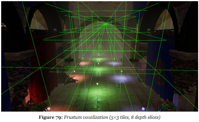
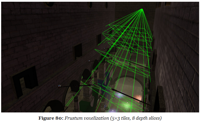
Clustered shading expands on the idea of tiled rendering but adds a segmentation on the 3rd axis. The “clustering” is done in view space, by splitting the frustum into a 3D grid.
-
Clustered Shading enables using normal information to perform per-cluster back-face culling of lights, again reducing the number of lighting computations.
-
Clustered Shading vs Tiled Shading :
-
We also show that Clustered Shading not only outperforms tiled shading in many scenes, but also exhibits better worst case behaviour under tricky conditions (e.g. when looking at high-frequency geometry with large discontinuities in depth).
-
Additionally, Clustered Shading enables real-time scenes with two to three orders of magnitudes more lights than previously feasible (up to around one million light sources).
-
Our implementation shows much less view-dependent performance, and is much faster for some cases that are challenging for tiled shading.
-
Compared to tiled shading, clusters generally are smaller, and therefore will be affected by fewer light sources.
-
Our implementation shows that both clustered deferred and forward shading offer real-time performance and can scale up to 1M lights. In addition, overhead for the clustering is low, making it competitive even for few lights.
-
The shading cost is proportional to the light density.
-
-
Clustered Forward vs Clustered Deferred :
-
Clustered Shading is really decoupled from the choice between deferred or forward rendering. It works with both, so you’re not locked into one or the other. This way you can make an informed choice between the two approaches based on other factors, such as whether you need custom materials and lighting models, or need deferred effects such as screen-space decals, or simply based on performance.
-
Godot
-
Clustered lighting uses a compute shader to group lights into a 3D frustum aligned grid.
-
At render time, pixels can lookup what lights affect the grid cell they are in and only run light calculations for lights that might affect that pixel.
-
This approach can greatly speed up rendering performance on desktop hardware, but is substantially less efficient on mobile.
-
There's a default limit of 512 clustered elements that can be present in the current camera view.
-
A clustered element is an omni light, a spot light, a decal or a reflection probe.
-
This limit can be increased by adjusting Max Clustered Elements in Project Settings > Rendering > Limits > Cluster Builder.
-
High-level overview
-
Build the clustering data structure.
-
Render scene to Z Pre-pass.
-
Find visible clusters.
-
Reduce repeated values in the list of visible clusters.
-
Perform light culling and assign lights to clusters.
-
Shade samples using light list.
-
Steps two and six won’t be covered since they are mostly dependent on the shading model you’re using.
-
Steps three and four are combined into one and covered in the section on Determining Active Clusters, much like in Van Oosten’s implementation .
Building the Cluster Grid
-
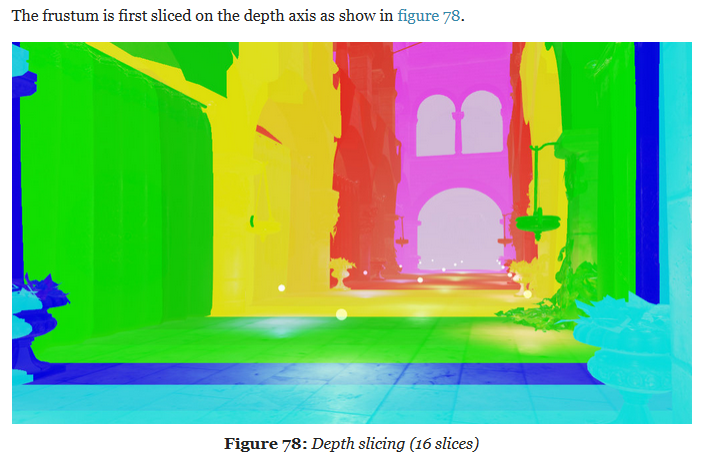
Depth Slicing :
-
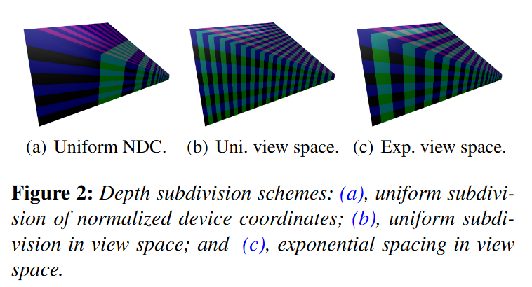
We’ll be focusing on building cluster grids that group samples based on their view space position. We’ll begin by tiling the view frustum exactly the same way you would in tiled shading and then subdividing it along the depth axis multiple times.
-
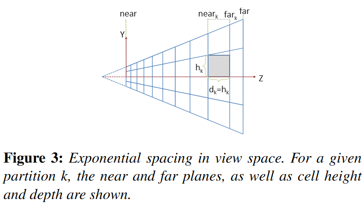
We choose to perform the subdivision in view space, by spacing the divisions exponentially to achieve self-similar subdivisions, such that the clusters become as cubical as possible (Figures 2(c) and 3).
-
 .
.
-
In Figure 3, we illustrate the subdivisions of a frustum. The number of subdivisions in the Y direction (Sy) is given in screen space (e.g. to form tiles of 32×32 pixels).
-
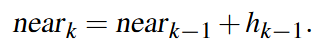
The near plane for a division k, near k, can be calculated from:
-
 .
.
-
 .
.
-
"I settled on a 16x9x24 subdivision because it matches my monitors aspect ratio, but it honestly could have been something else." - Angel Ortiz.
-
Doom (2016) :
-
Uses the one below, which doesn't represent any of the three above.
-
 .
.
-
Solving:
 .
.
-
The major advantage of the equation above is that the only variable is Z and everything else is a constant.
-
 .
.
-
-
Avalanche Studios :
-
Another option we have considered, but not yet explored, is to not base it on pixel count, but simply divide the screen into a specific number of tiles regardless of resolution. This may reduce coherency on the GPU side somewhat in some cases, but would also decouple the CPU workload from the GPU workload and allow for some useful CPU side optimizations if the tile counts are known at compile time.
-
We are using exponential depth slicing, much like in the paper. There is nothing dictating that this is what we have to use, or for that matter that it is the best or most optimal depth slicing strategy; however, the advantage is that the shape of the clusters remain the same as we go deeper into the depth. On the other hand, clusters get larger in world space, which could potentially result in some distant clusters containing a much larger amount of lights. Depending on the game, it may be worth exploring other options.
-
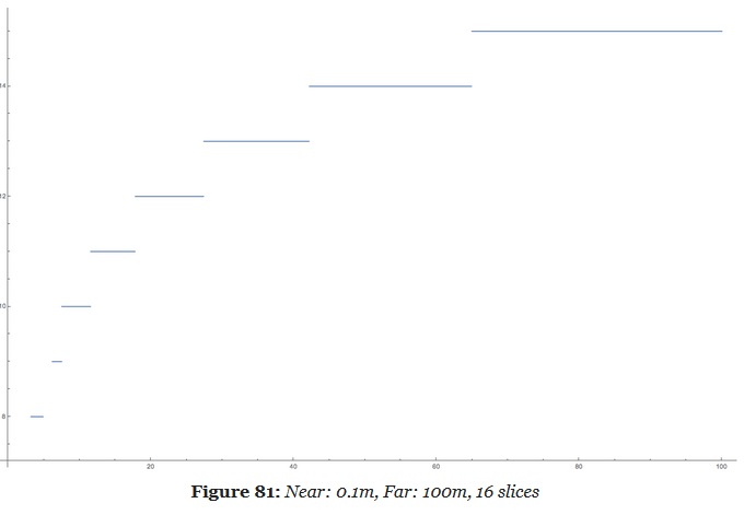
Our biggest problem was that our depth ratio is massive, with near plane as close as 0.1m and far plane way out on the other side of the map, at 50,000m. This resulted in poor utilization of our limited depth slices, currently 16 of them. The step from one slice to the next is very large. Fortunately, in our game we don’t have any actual light sources beyond a distance of 500m. So we simply decided to keep our current distant light system for distances beyond 500m and limit the far range for clustering to that.
-
 .
.
-
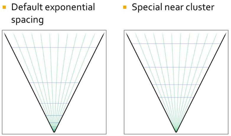
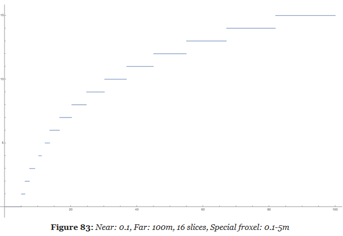
This improved the situation notably, but was still not ideal. We still burnt half of our slices on the first 7 meters from the camera. Given how our typical scenes look like, that’s likely going to be mostly empty space in most situations. So to improve the situation, we made the first slice special and made that go from near plane to an arbitrary visually tweaked distance, currently 5m. This gave us much better utilization.
-
-
Filament Engine :
-
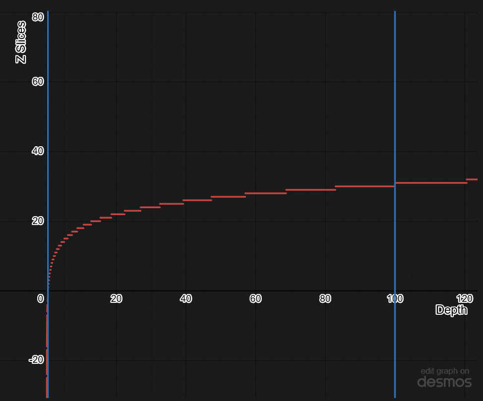
The depth slicing is not linear, but exponential. In a typical scene, there will be more pixels close to the near plane than to the far plane. An exponential grid of froxels will therefore improve the assignment of lights where it matters the most.
-
 .
.
-
A simple exponential voxelization is unfortunately not enough. The graphic above clearly illustrates how world space is distributed across slices but it fails to show what happens close to the near plane.
-
A simple exponential distribution uses up half of the slices very close to the camera. In this particular case, we use 8 slices out of 16 in the first 5 meters. Since dynamic world lights are either point lights (spheres) or spot lights (cones), such a fine resolution is completely unnecessary so close to the near plane.
-
Our solution is to manually tweak the size of the first froxel depending on the scene and the near and far planes. By doing so, we can better distribute the remaining froxels across the frustum.
-
 .
.
-
This new distribution is much more efficient and allows a better assignment of the lights throughout the entire frustum.
-
 .
.
-
We call a froxel a voxel in frustum space.
-
The frustum voxelization can be executed only once by a first compute shader (as long as the projection matrix does not change).
-
-
-
Screen Slicing :
-
Filament Engine :
-
1280x720px, 80x80px tiles.
-
-
-
-
 .
.
-
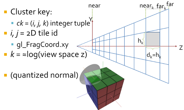
Cluster assignments is a simple mapping from sample coordinate, to an integer tuple
i,j,k. -
iandjare the tile coordinates, which can be derived by dividinggl_FragCoord.xyby the tile size.-
i = bx_screen_space/txcj = by_screen_space/tyc.
-
-
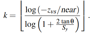
kis a logarithmic function of the view space Z of the sample, not simply the logarithm.-
The logarithmic subdivisions also means that as clusters become larger further away, we get a kind of LOD behaviour and do not end up with insane numbers of clusters, for a wide range of view parameters.
-
-
We use this subdivision as it creates self similar clusters that are as cube like as possible. This makes them better suited for culling.
-
 .
.
-
An easy solution is to use Axis Aligned Bounding Boxes (AABB) that enclose each cluster. AABBs built from the max and min points of the clusters will be ever so slightly larger than the actual clusters. We’re okay with this since it ensures that there are no gaps in between volumes due to precision issues. Also, AABB’s can be stored using only only two vec3’s, a max and min point.
-
This compute shader is ran once per cluster and aims to obtain the min and max points of the AABB encompassing said cluster.
-
First, imagine we’re looking at the view frustum from a front camera perspective, like we did in the Tiled Shading animations of part one. Each tile will have a min and max point, which in our coordinate system will be the upper right and bottom left vertices of a tile respectively. After obtaining these two points in screen space we set their Z position equal to the near plane, which in NDC and in my specific setup is equal to -1.
-
I know, I know. I should be using reverse Z, not the default OpenGL layout, I’ll fix that eventually.
-
-
Then, we transform these min and max points to view space. Next, we obtain the Z value of the “near” and “far” plane of our target mini-frustum / cluster. And, armed with the knowledge that all rays meet at the origin in view space, a pair of min and max values in screen space and both bounding planes of the cluster, we can obtain the four points intersecting those planes that will represent the four corners of the AABB encompassing said cluster. Lastly, we find the min and max of those points and save their values to the cluster array. And voilà, the grid is complete!
-
Screen To View:
-
Converts a given point in screen space to view space by taking the reverse transformation steps taken by the graphics pipeline.
-
-
Line Intersection to Z Plane:
-
Used to obtain the points on the corners of the AABB that encompasses a cluster. The normal vector of the planes is fixed at 1.0 in the z direction because we are evaluating the points in view space and positive z points towards the camera from this frame of reference.
-
-
When to recalculate:
-
Our list of cluster AABBs will be valid as long as the view frustum stays the same shape. So, it can be calculated once at load time and only recalculated with any changes in FOV or other view field altering camera properties.
-
My initial profiling in RenderDoc seems to indicate that the GPU can run this shader really quickly, so I think it wouldn’t be a huge deal either if this was done every frame.
-
Idk
-
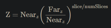
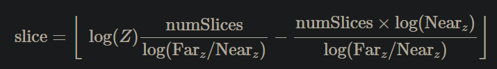
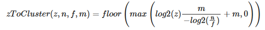
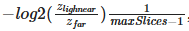
From depth to froxel :
-
Given a near plane $n$, a far plane $m$, a maximum number of depth slices $z$ and a linear depth value in the range
[0..1], this equation can be used to compute the index of the cluster for a given position. -
 .
.
-
This formula suffers however from the resolution issue mentioned previously. We can fix it by introducing $sn$, a special near value that defines the extent of the first froxel (the first froxel occupies the range
[n..sn], the remaining froxels[sn..f]). -
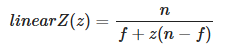
The following equation can be used to compute a linear depth value from
gl_FragCoord.z(assuming a standard OpenGL projection matrix). -
 .
.
-
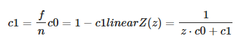
This equation can be simplified by pre-computing two terms $c0$ and $c1$:
-
 .
.
-
This simplification is important because we will pass the linear $z$ value to a
log2. Since the division becomes a negation under a logarithmic, we can avoid a division by using-log2(z * c0 + c1)instead. -
Implementation to compute a froxel index from a fragment's screen coordinates:
#define MAX_LIGHT_COUNT 16 // max number of lights per froxel uniform uvec4 froxels; // res x, res y, count y, count y uniform vec4 zParams; // c0, c1, index scale, index bias uint getDepthSlice() { return uint(max(0.0, log2(zParams.x * gl_FragCoord.z + zParams.y) * zParams.z + zParams.w)); } uint getFroxelOffset(uint depthSlice) { uvec2 froxelCoord = uvec2(gl_FragCoord.xy) / froxels.xy; froxelCoord.y = (froxels.w - 1u) - froxelCoord.y; uint index = froxelCoord.x + froxelCoord.y * froxels.z + depthSlice * froxels.z * froxels.w; return index * MAX_FROXEL_LIGHT_COUNT; } uint slice = getDepthSlice(); uint offset = getFroxelOffset(slice); // Compute lighting...-
Several uniforms must be pre-computed to perform the index evaluation efficiently.
froxels[0] = TILE_RESOLUTION_IN_PX; froxels[1] = TILE_RESOLUTION_IN_PX; froxels[2] = numberOfTilesInX; froxels[3] = numberOfTilesInY; zParams[0] = 1.0f - Z_FAR / Z_NEAR; zParams[1] = Z_FAR / Z_NEAR; zParams[2] = (MAX_DEPTH_SLICES - 1) / log2(Z_SPECIAL_NEAR / Z_FAR); zParams[3] = MAX_DEPTH_SLICES; -
-
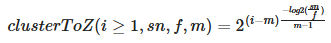
From froxel to depth :
-
 .
.
-
For $i = 0$, the z value is 0. The result of this equation is in the
[0..1]range and should be multiplied by $f$ to get a distance in world units. -
The compute shader implementation should use
exp2instead of apow. The division can be precomputed and passed as a uniform.
-
Data Structure
-
They’re implemented solely on the GPU using shader storage buffer objects, so keep in mind that reads and writes have incoherent memory access and will require the appropriate barriers to avoid any disasters.
-
 .
.
-
"At the end, you get an accelerated structure like this, which is just a grid where you can look up your light lists."
-
-
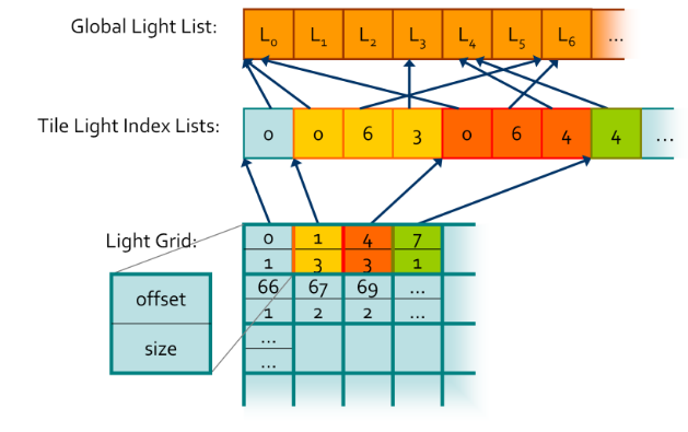
Global Light List :
-
It is an array containing all of the lights in a given scene with a size equivalent to the maximum amount of lights possible in the scene.
-
-
Global Light Index List :
-
Every light will have its own unique index based on its location in the Global Light List and that index is stored in the Global Light Index List.
-
This array contains the indices of all of the active lights in the scene grouped by cluster.
-
-
Light Grid :
-
Contain information as to how these indices relate to their parent clusters.
-
This array has as many elements as there are clusters and each element contains two unsigned ints, one that stores the offset to the Global Light Index List and another that contains the number of lights intersecting the cluster.
-
Each cell stores an offset and count that represent a range in ?.
-
This range contains a list of light indices indicating all the lights that the may affect the samples in the tile.
-
The Light Grid provides access to light list for each pixel.
-
-
Unlike what’s shown in the diagram, the global light index list does not necessarily store the indices for each cluster sequentially, in fact, it might store them in a completely random order.
-
If you’re wondering why we need such a convoluted data structure, the quick answer is that it plays nicely with the GPU and works well in parallel. Also, it allows both compute shaders and pixel shaders to read the same data structure and execute the same code. Lastly, it is pretty memory efficient since clusters tend to share the same lights and by storing indices to the global light list instead of the lights themselves we save up memory.
-
-
Check lights against every cluster of the view frustum. Performs light culling for every cluster in the cluster grid.
-
Thread groups sizes are actually relevant in this compute shader since I’m using shared GPU memory to reduce the number of reads and writes by only loading each light once per thread group, instead of once per cluster.
-
First, each thread gets its bearings and begins by calculating some initialization values.
-
For example, how many threads there are in a thread group, what it’s linear cluster index is and in how many passes it shall traverse the global light list.
-
-
Next, each thread initializes a count variable of how many lights intersect its cluster and a local index light array to zero.
-
Once setup is complete, each thread group begins a traversal of a batch of lights. Each individual thread will be responsible for loading a light and writing it to shared memory so other threads can read it.
-
A barrier after this step ensures all threads are done loading before continuing.
-
Then, each thread performs collision detection for its cluster, using the AABB we determined in step one, against every light in the shared memory array, writing all positive intersections to the local thread index array.
-
We repeat these steps until every light in the global light array has been evaluated.
-
Next, we atomically add the local number of active lights in a cluster to the globalIndexCount and store the global count value before we add to it.
-
This number is our offset to the global light index list and due to the nature of atomic operations we know that it will be unique per cluster , since only one thread has access to it at any given time.
-
Then, we populate the global light index list by transferring the values from the local light index list (named visibleLightIndices in the code) into the global light index list starting at the offset index we just obtained.
-
Finally, we write the offset value and the count of how many lights intersected the cluster to the lightGrid array at the given cluster index.
-
-
Once this shader is done running the data structures will contain all of the values necessary for a pixel shader to read the list of lights that are affecting a given fragment, since we can use the getClusterIndex function from the previous section to find which cluster a fragment belongs to.
-
With this, we’ve completed step five and therefore have all the building blocks in place for a working clustered shading implementation.
-
Even this simple culling method will still manage lights in the order of tens of thousands.
-
Extra Optimizations :
-
Jeremiah Van Oosten’s thesis writes about optimizing Clustered Renderers and has links to his testing framework where you can compare different efficient rendering algorithms.
-
He goes into detail as to how spatial optimization structures like Boundary Volume Hierarchies (BVH) and efficient light sorting can significantly increase performance and allow for scenes with millions of dynamic light sources in real-time.
-
Right now, it seems that implementing the BVH will be my first task — and specially after how important being familiar with BVH’s will become after Turing.
-
-
virtual shadow mapping enables hundreds of real-time shadow casting dynamic lights.
-
It should be considered an alternate clustering method best suited for mobile hardware.
-
Doom 2016 goes into optimized shaders to make use of GCN scalar units and saved some Vector General-Purpose Registers(VGPR). Also, by voxelizing environment probes, decals and lights the benefits of the cluster data structure were brought over to nearly all items that influence lighting.
-
-
Avalanche Studios :
-
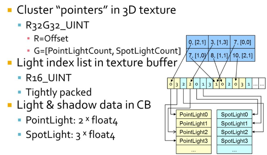
Given a screen position and a depth value (whether from a depth buffer or the rasterized depth in a forward pass) we start by looking up the cluster from a 3D texture. Each texel represents a cluster and its light list.
-
The red channel gives us an offset to where the light list starts, whereas the green channel contains the light counts. The light lists are then stored in a tightly packed lists of indexes to the lights. The actual light source data is stored as arrays in a constant buffer.
-
All in all the data structure is very compact. In a typical artists lit scene it may be around 50- 100kb of data to upload to the GPU every frame.
-
 .
.
-
Data coherency :
-
So the difference between tiled and clustered is that we pick a light list on a per-pixel basis instead of per-tile, depending on which cluster we fall within. Obviously though, in a lot of cases nearby pixels will choose the same light list, in particular neighbors within the same tile on a similar depth. If we visualize what light lists were chosen, we can see that there are a bunch of different paths taken beyond just the tile boundaries. A number of depth discontinuities from the foliage in front of the player gets clearly visible. This may seem like a big problem, but here we are only talking about fetching different data. This is not a problem for a GPU, it’s something they do all the time for regular texture fetches, and this is even much lower frequency than that.
-
-
-
Filament Engine :
-
The list of lights per froxel can be passed to the fragment shader either as an SSBO or a texture.
-
During the rendering pass, we can compute the ID of the froxel a fragment belongs to and therefore the list of lights that can affect that fragment.
-
Finding Active Clusters / Unique Clusters
-
Motivation :
-
This section is optional since active cluster determination is not a crucial part of light culling.
-
Even though it isn’t terribly optimal, you can simply perform culling checks for all clusters in the cluster grid every frame.
-
Thankfully, determining active clusters doesn’t take much work to implement and can speed up the light culling pass considerably.
-
The only drawback is that it will require a Depth Pre-pass .
-
-
Depth Pre-pass :
-
The depth map generated is used to determine the minimum and maximum depth values within a tile, that is the minimum and maximum depths across the entire tile.
-
-
The key idea is that not all clusters will be visible all of the time, and there is no point in performing light culling against clusters you cannot see.
-
So, we can check every pixel in parallel for their cluster ID and mark it as active on a list of clusters.
-
This list will most likely be sparsely populated, so we will compact it into another list using atomic operations.
-
Then, during light culling we will check light “collisions” against the compacted list instead, saving us from having to check every light for every cluster.
-
To increase efficiency, both Van Oosten and Olsson compact this list into a set of unique clusters .
-
We compact the grid into the list of non-zero elements.
-
This leaves us with a list of clusters which needs lights assigned to them.
-
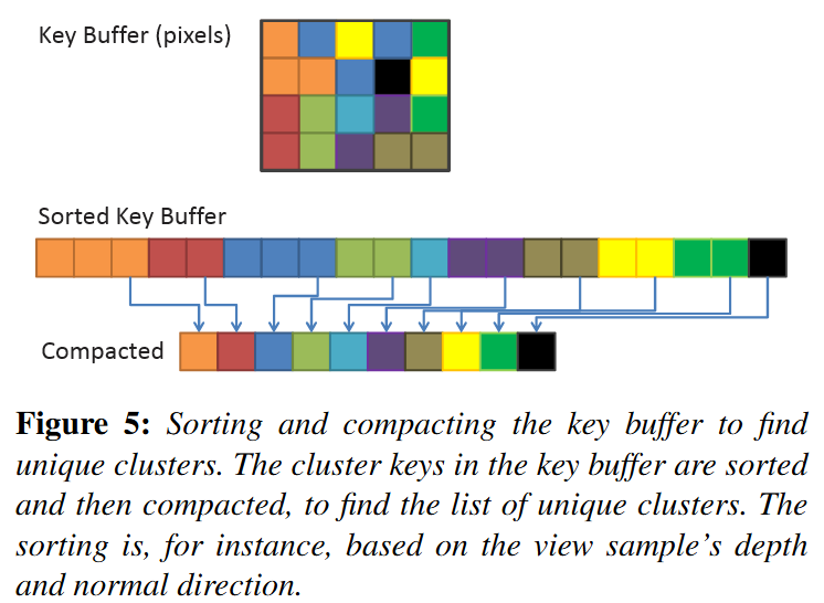
The most obvious method to find the unique clusters in parallel is to simply sort the cluster keys, and then perform a compaction step that removes any with an identical neighbour .
-
 .
.
-
-
Identifying unique clusters :
-
Local Sorting
-
We sort samples in each screen space tile locally. This allows us to perform the sorting operation in on-chip shared memory, and use local (and therefore smaller) indices to link back to the source pixel.
-
We extract unique clusters from each tile using a parallel compaction. From this, we get the globally unique list of clusters. During the compaction, we also compute and store a link from each sample to its associated cluster.
-
-
Page Tables-
The second technique is similar to the page table approach used by virtual textures (Section 2). However, as the range of possible cluster keys is very large, we cannot use a direct mapping between cluster key and physical storage location for the cluster data; it simply would typically not fit into GPU memory. Instead we use a virtual mapping, and allocate physical pages where any actual keys needs storage. Lefohn et.al. [LSK∗06] provide details on software GPU implementation of virtual address translation. We exploit the fact that all physical pages are allocated in a compact range, and we can therefore compact that range to find the unique clusters.
-
-
Other methods:-
Both sorting and compaction are relatively efficient and readily available GPU building blocks. However, despite steady progress, sorting remains an expensive operation.
-
Methods that rely on adjacent screen-space coherency are not robust, especially with respect to stochastic frame buffers.
-
We therefore focus on techniques that do not suffer from this weaknesses.
-
-
-
Explicit Bounds :
-
As the actual view-sample positions and normals typically have tighter bounds, we also evaluate explicit 3D bounds and normal cones.
-
We compute the explicit bounds by performing a reduction over the samples in each cluster (e.g., we perform a min-max reduction to find the AABB enclosing each cluster).
-
The results of the reduction are stored separately in memory.
-
When using page tables, the reduction is difficult to implement efficiently, because of the many-to-one mapping from view samples to cluster data, we would need to make use of atomic operations, and get a high rate of collisions. We deemed this to be impractically expensive.
-
We therefore only implement explicit bounds for local sort.
-
After the local sort, information about which samples belong to a given cluster is readily available.
-
-
//Input
vec2 pixelID; // The thread x and y id corresponding to the pixel it is representing
vec2 screenDimensions; // The total pixel size of the screen in x and y

//Output
bool clusterActive[];

//We will evaluate the whole screen in one compute shader
//so each thread is equivalent to a pixel
void markActiveClusters(){
    //Getting the depth value
    vec2 screenCord = pixelID.xy / screenDimensions.xy;
    float z = texture(screenCord) //reading the depth buffer

    //Getting the linear cluster index value
    uint clusterID = getClusterIndex(vec3(pixelID.xy, z));
    clusterActive[clusterID] = true;
}
//Input
vec3 pixelCoord;  // Screen space pixel coordinate with depth
uint tileSizeInPx; // How many pixels a rectangular cluster takes in x and y
uint3 numClusters; // The fixed number of clusters in x y and z axes

//Output
uint clusterIndex; // The linear index of the cluster the pixel belongs to

uint getClusterIndex(vec3 pixelCoord){
    // Uses equation (3) from Building a Cluster Grid section
    uint clusterZVal  = getDepthSlice(pixelCoord.z);

    uvec3 clusters    = uvec3( uvec2( pixelCoord.xy / tileSizeInPx), clusterZVal);
    uint clusterIndex = clusters.x +
                        numClusters.x * clusters.y +
                        (numClusters.x * numClusters.y) * clusters.z;
    return clusterIndex;
}
//Input
bool clusterActive[]; //non-compacted list
uint globalActiveClusterCount; //Number of active clusters

//Output
uint uniqueActiveClusters[]; //compacted list of active clusters

//One compute shader for all clusters, one cluster per thread
void buildCompactClusterList(){
    uint clusterIndex  = gl_GlobalInvocationID;
    if(clusterActive[clusterIndex]){
       uint offset = atomicAdd(globalActiveClusterCount, 1);
       uniqueActiveClusters[offset] = clusterIndex;
    }
}
Light Culling / Light Assignment
-
This step aims to assign lights to each cluster based on their view space position.
-
The main idea is that we perform something very similar to a “light volume collision detection” against the active clusters in the scene and append any lights within a cluster to a local list of lights.
-
Performing this “light volume collision detection” requires that I define clearly what I mean by light volume .
-
In a nutshell, lights become dimmer with distance. After a certain point they are so dim we can assume they aren’t contributing to shading anymore so, we mark those points as our boundary. The volume contained within the boundary is our light volume and if that volume intersects with the AABB of a cluster, we assume that light is contained within the cluster.
//Input:
uint light; // A given light index in the shared lights array
uint tile;  // The cluster index we are testing

//Checking for intersection given a cluster AABB and a light volume
bool testSphereAABB(uint light, uint tile){
    float radius = sharedLights[light].range;
    vec3 center  = vec3(viewMatrix * sharedLights[light].position);
    float squaredDistance = sqDistPointAABB(center, tile);

    return squaredDistance <= (radius * radius);
}
-
The main idea is that we check the distance between the point light sphere center and the AABB. If the distance is less than the radius they are intersecting.
-
For spotlights, the light volume and consequently the collision tests will be very different.
-
Check out this presentation by Emil Persson that explains how they implemented spotlight culling in Just Cause 3 if you do want to know more.
-
Light Assignment
-
The lights have a limited range, with some falloff which goes to 0 at the boundary.
-
There is no pre-computation so all geometry and lights are allowed to change freely from frame to frame.
-
The goal of the light assignment stage is to calculate the list of lights influencing each cluster. Previous designs for tiled deferred shading implementations have by and large utilized a brute force approach to finding the intersection between lights and tiles. That is, light-cluster overlaps were found by, for each tile, iterating over all lights in the scene and testing bounding volumes. This is tolerable for reasonably low numbers of lights and clusters.
-
To support large numbers of lights and a dynamically varying number of clusters, we use a fully hierarchical approach based on a spatial tree over the lights.
-
Each frame, we construct a bounding volume hierarchy (BVH) by first sorting the lights according to the Z-order (Morton Code) based on the discretized centre position of each light. We derive the discretization from a dynamically computed bounding volume around all lights.
-
We use a BVH with a branching factor of 32, which is rebuilt each frame.
-
When not so many lights are used, there are many other approaches which may be better.
-
-
The leaves of the search tree we get directly from the sorted data.
-
Next, 32 consecutive leaves are grouped into a bounding volume (AABB) to form the first level above the leaves.
-
The next level is constructed by again combining 32 consecutive elements. We continue until a single root element remains.
-
For each cluster, we traverse this BVH using depth-first traversal. At each level, the bounding box of the cluster (either explicitly computed from the cluster’s contents or implicitly derived from the cluster’s key) is tested against the bounding volumes of the child nodes. For the leaf nodes, the sphere bounding the light source is used; other nodes store an AABB enclosing the node. The branching factor of 32 allows efficient SIMD-traversal on the GPU and keeps the search tree relatively shallow (up to 5 levels), which is used to avoid expensive recursion (the branching factor should be adjusted depending on the GPU used, the factor of 32 is convenient on current NVIDIA GPUs).
-
If a normal cone is available for a cluster, we use this cone to further reject lights that will not affect any samples in the cluster; etc (to summarize).
-
Avalanche Studios :
-
Deriving the explicit cluster bounds was something that could be interesting, but we found that sticking to implicit bounds simplified the technique, while also allowing the light assignment to run on the CPU.
-
In addition, this gives us scene independence. This means that we don’t need to know what the scene looks like to fill in the clusters, and this also allows us to evaluate light at any given point in space, even if it’s floating in thin air. This could be relevant for instance for ray-marching effects.
-
Given that we are doing the light assignment on the CPU, one may suspect that this will become a significant burden for the CPU. However, our implementation is fast enough to actually save us a bunch of CPU time over our previous solution. In a normal artist lit scene we recorded 0.1ms on one core for clustered shading. The old code supporting our previous forward pass for transparency that was still running in our system was still consuming 0.67ms for the same scene, a cost that we can now eliminate.
-
-
Filament Engine :
-
Before rendering a frame, each light in the scene is assigned to any froxel it intersects with. The result of the lights assignment pass is a list of lights for each froxel.
-
Lights assignment can be done in two different ways, on the GPU or on the CPU.
-
On GPU:
-
The lights are stored in Shader Storage Buffer Objects (SSBO) and passed to a compute shader that assigns each light to the corresponding froxels.
-
The lights assignment can be performed each frame by another compute shader.
-
The threading model of compute shaders is particularly well suited for this task. We simply invoke as many workgroups as we have froxels (we can directly map the X, Y and Z workgroup counts to our froxel grid resolution). Each workgroup will in turn be threaded and traverse all the lights to assign.
-
Intersection tests imply simple sphere/frustum or cone/frustum tests.
-
Assigning Lights with Froxels :
-
Assigning lights to froxels can be implemented on the GPU using two compute shaders.
-
The first one, creates the froxels data (4 planes + a min Z and max Z per froxel) in an SSBO and needs to be run only once.
-
Projection matrix
-
The projection matrix used to render the scene (view space to clip space transformation).
-
-
Inverse projection matrix
-
The inverse of the projection matrix used to render the scene (clip space to view space transformation).
-
-
Depth parameters
-
 , maximum number of depth slices, Z near and Z far.
-
-
Clip space size
-
 , with $F_x$ the number of tiles on the X axis, $F_r$ the resolution in pixels of a tile and w the width in pixels of the render target.
-
-
#version 310 es precision highp float; precision highp int; #define FROXEL_RESOLUTION 80u layout(local_size_x = 1, local_size_y = 1, local_size_z = 1) in; layout(location = 0) uniform mat4 projectionMatrix; layout(location = 1) uniform mat4 projectionInverseMatrix; layout(location = 2) uniform vec4 depthParams; // index scale, index bias, near, far layout(location = 3) uniform float clipSpaceSize; struct Froxel { // NOTE: the planes should be stored in vec4[4] but the // Adreno shader compiler has a bug that causes the data // to not be read properly inside the loop vec4 plane0; vec4 plane1; vec4 plane2; vec4 plane3; vec2 minMaxZ; }; layout(binding = 0, std140) writeonly restrict buffer FroxelBuffer { Froxel data[]; } froxels; shared vec4 corners[4]; shared vec2 minMaxZ; vec4 projectionToView(vec4 p) { p = projectionInverseMatrix * p; return p / p.w; } vec4 createPlane(vec4 b, vec4 c) { // standard plane equation, with a at (0, 0, 0) return vec4(normalize(cross(c.xyz, b.xyz)), 1.0); } void main() { uint index = gl_WorkGroupID.x + gl_WorkGroupID.y * gl_NumWorkGroups.x + gl_WorkGroupID.z * gl_NumWorkGroups.x * gl_NumWorkGroups.y; if (gl_LocalInvocationIndex == 0u) { // first tile the screen and build the frustum for the current tile vec2 renderTargetSize = vec2(FROXEL_RESOLUTION * gl_NumWorkGroups.xy); vec2 frustumMin = vec2(FROXEL_RESOLUTION * gl_WorkGroupID.xy); vec2 frustumMax = vec2(FROXEL_RESOLUTION * (gl_WorkGroupID.xy + 1u)); corners[0] = vec4( frustumMin.x / renderTargetSize.x * clipSpaceSize - 1.0, (renderTargetSize.y - frustumMin.y) / renderTargetSize.y * clipSpaceSize - 1.0, 1.0, 1.0 ); corners[1] = vec4( frustumMax.x / renderTargetSize.x * clipSpaceSize - 1.0, (renderTargetSize.y - frustumMin.y) / renderTargetSize.y * clipSpaceSize - 1.0, 1.0, 1.0 ); corners[2] = vec4( frustumMax.x / renderTargetSize.x * clipSpaceSize - 1.0, (renderTargetSize.y - frustumMax.y) / renderTargetSize.y * clipSpaceSize - 1.0, 1.0, 1.0 ); corners[3] = vec4( frustumMin.x / renderTargetSize.x * clipSpaceSize - 1.0, (renderTargetSize.y - frustumMax.y) / renderTargetSize.y * clipSpaceSize - 1.0, 1.0, 1.0 ); uint froxelSlice = gl_WorkGroupID.z; minMaxZ = vec2(0.0, 0.0); if (froxelSlice > 0u) { minMaxZ.x = exp2((float(froxelSlice) - depthParams.y) * depthParams.x) * depthParams.w; } minMaxZ.y = exp2((float(froxelSlice + 1u) - depthParams.y) * depthParams.x) * depthParams.w; } if (gl_LocalInvocationIndex == 0u) { vec4 frustum[4]; frustum[0] = projectionToView(corners[0]); frustum[1] = projectionToView(corners[1]); frustum[2] = projectionToView(corners[2]); frustum[3] = projectionToView(corners[3]); froxels.data[index].plane0 = createPlane(frustum[0], frustum[1]); froxels.data[index].plane1 = createPlane(frustum[1], frustum[2]); froxels.data[index].plane2 = createPlane(frustum[2], frustum[3]); froxels.data[index].plane3 = createPlane(frustum[3], frustum[0]); froxels.data[index].minMaxZ = minMaxZ; } }-
The second compute shader, runs every frame (if the camera and/or lights have changed) and assigns all the lights to their respective froxels.
-
Light index buffer
-
For each froxel, the index of each light that affects said froxel. The indices for point lights are written first and if there is enough space left, the indices for spot lights are written as well. A sentinel of value 0×7fffffffu separates point and spot lights and/or marks the end of the froxel's list of lights. Each froxel has a maximum number of lights (point + spot).
-
-
Point lights buffer
-
Array of structures describing the scene's point lights.
-
-
Spot lights buffer
-
Array of structures describing the scene's spot lights.
-
-
Froxels buffer
-
The list of froxels represented by planes, created by the previous compute shader.
-
-
#version 310 es precision highp float; precision highp int; #define LIGHT_BUFFER_SENTINEL 0x7fffffffu #define MAX_FROXEL_LIGHT_COUNT 32u #define THREADS_PER_FROXEL_X 8u #define THREADS_PER_FROXEL_Y 8u #define THREADS_PER_FROXEL_Z 1u #define THREADS_PER_FROXEL (THREADS_PER_FROXEL_X * \ THREADS_PER_FROXEL_Y * THREADS_PER_FROXEL_Z) layout(local_size_x = THREADS_PER_FROXEL_X, local_size_y = THREADS_PER_FROXEL_Y, local_size_z = THREADS_PER_FROXEL_Z) in; // x = point lights, y = spot lights layout(location = 0) uniform uvec2 totalLightCount; layout(location = 1) uniform mat4 viewMatrix; layout(binding = 0, packed) writeonly restrict buffer LightIndexBuffer { uint index[]; } lightIndexBuffer; struct PointLight { vec4 positionFalloff; // x, y, z, falloff vec4 colorIntensity; // r, g, b, intensity vec4 directionIES; // dir x, dir y, dir z, IES profile index }; layout(binding = 1, std140) readonly restrict buffer PointLightBuffer { PointLight lights[]; } pointLights; struct SpotLight { vec4 positionFalloff; // x, y, z, falloff vec4 colorIntensity; // r, g, b, intensity vec4 directionIES; // dir x, dir y, dir z, IES profile index vec4 angle; // angle scale, angle offset, unused, unused }; layout(binding = 2, std140) readonly restrict buffer SpotLightBuffer { SpotLight lights[]; } spotLights; struct Froxel { // NOTE: the planes should be stored in vec4[4] but the // Adreno shader compiler has a bug that causes the data // to not be read properly inside the loop vec4 plane0; vec4 plane1; vec4 plane2; vec4 plane3; vec2 minMaxZ; }; layout(binding = 3, std140) readonly restrict buffer FroxelBuffer { Froxel data[]; } froxels; shared uint groupLightCounter; shared uint groupLightIndexBuffer[MAX_FROXEL_LIGHT_COUNT]; float signedDistanceFromPlane(vec4 p, vec4 plane) { // plane.w == 0.0, simplify computation return dot(plane.xyz, p.xyz); } void synchronize() { memoryBarrierShared(); barrier(); } void main() { if (gl_LocalInvocationIndex == 0u) { groupLightCounter = 0u; } memoryBarrierShared(); uint froxelIndex = gl_WorkGroupID.x + gl_WorkGroupID.y * gl_NumWorkGroups.x + gl_WorkGroupID.z * gl_NumWorkGroups.x * gl_NumWorkGroups.y; Froxel current = froxels.data[froxelIndex]; uint offset = gl_LocalInvocationID.x + gl_LocalInvocationID.y * THREADS_PER_FROXEL_X; for (uint i = 0u; i < totalLightCount.x && groupLightCounter < MAX_FROXEL_LIGHT_COUNT && offset + i < totalLightCount.x; i += THREADS_PER_FROXEL) { uint currentLight = offset + i; vec4 center = pointLights.lights[currentLight].positionFalloff; center.xyz = (viewMatrix * vec4(center.xyz, 1.0)).xyz; float r = inversesqrt(center.w); if (-center.z + r > current.minMaxZ.x && -center.z - r <= current.minMaxZ.y) { if (signedDistanceFromPlane(center, current.plane0) < r && signedDistanceFromPlane(center, current.plane1) < r && signedDistanceFromPlane(center, current.plane2) < r && signedDistanceFromPlane(center, current.plane3) < r) { uint index = atomicAdd(groupLightCounter, 1u); groupLightIndexBuffer[index] = currentLight; } } } synchronize(); uint pointLightCount = groupLightCounter; offset = froxelIndex * MAX_FROXEL_LIGHT_COUNT; for (uint i = gl_LocalInvocationIndex; i < pointLightCount; i += THREADS_PER_FROXEL) { lightIndexBuffer.index[offset + i] = groupLightIndexBuffer[i]; } if (gl_LocalInvocationIndex == 0u) { if (pointLightCount < MAX_FROXEL_LIGHT_COUNT) { lightIndexBuffer.index[offset + pointLightCount] = LIGHT_BUFFER_SENTINEL; } } } -
-
-
On CPU:
-
The algorithm is different from the GPU implementation. Instead of iterating over every light for each froxel, the engine will “rasterize” each light as froxels. For instance, given a point light’s center and radius, it is trivial to compute the list of froxels it intersects with.
-
This technique has the added benefit of providing tighter culling than in the GPU variant. The CPU implementation can also more easily generate a packed list of lights.
-
-
Culling
-
Avalanche Studios :
-
Point light :
-
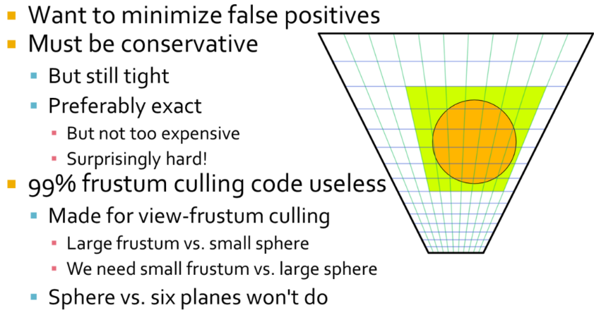 .
.
-
Our light sources are typically artist placed, scaled for human environments in an outdoor world, so generally speaking from meters to tens of meters. So a light source generally intersects many clusters. The typical sphere-frustum tests that you can find online are not suitable for this sort of culling. They are made for view-frustum culling and based on the assumption that the frustum typically is much larger than the sphere, which is the opposite of what we have here. Typically they simply test sphere vs plane for each six planes of the frustum. This is conservative, but lets through spheres that aren’t completely behind any of the planes, such as in the frustum corners. The result you get is that green rectangle, or essentially a ”cube” of clusters around the light. But that’s also the first thing we compute. We simply compute the screen-space and depth extents of the light analytically first, so this test doesn’t actually help anything at all after that.
-
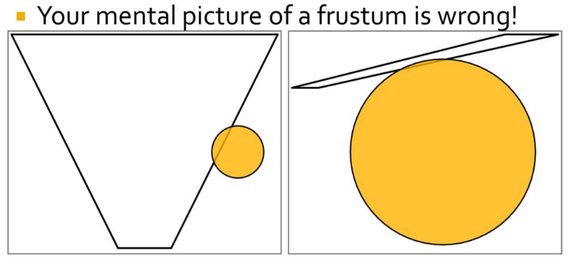 .
.
-
Most frustum culling code is written with the scenario on the left in mind. We need to handle the scenario on the right.
-
One way to go about frustum culling is testing all planes, all edges and all vertices. This would work, but be too costly to outweigh the gains from fewer false positives. A fast, conservative but relatively tight solution is what we are looking for. There are many approaches that seem fitting, but there are also many complications, which has ultimately thrown many of our attempts into the garbage bin. One relatively straightforward approach is to cull against the cluster’s AABB. This is fast and gives fairly decent results, but it’s possible to do better.
-
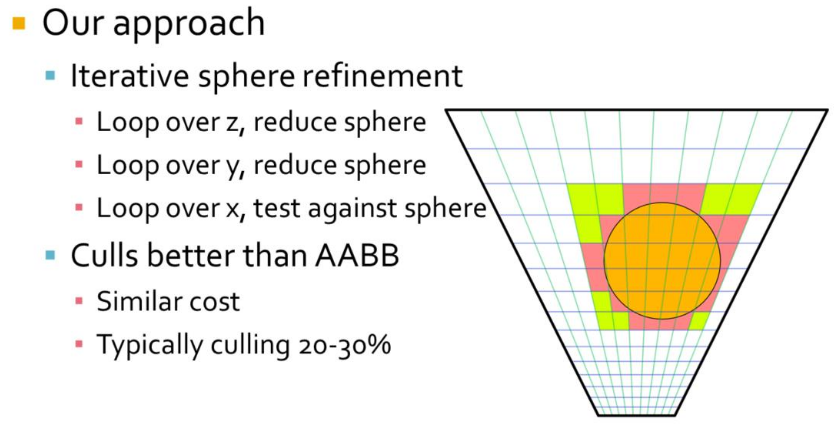
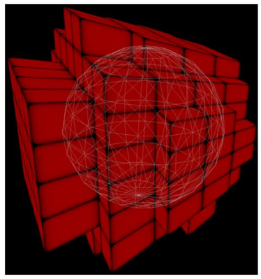 .
.
-
Starting with the ”cube” of clusters around the light, in our outer loop we iterate over the slices in z direction. We intersect the sphere with the slice where it is the widest. This results in a circle of a smaller radius than the original sphere, we thus continue in the y direction using a sphere of this smaller radius and the circle’s midpoint. In the center slice we simply proceed with the original sphere. We repeat this procedure in y and have an even smaller sphere. Then in the inner loop we do plane vs. sphere tests in x direction to get a strip of clusters to add the light to.
-
To optimize all the math we take advantage of the fact that in view-space, all planes will have components that are zero. A plane in the x direction will have zero y and offset, y direction has zero x and offset, and z-direction is basically only a z offset.
-
The resulting culling is somewhat tighter than a plain AABB test, and costs about the same. Where AABB culls around 15-25%, this technique culls around 20-30% from the “cube” of clusters.
-
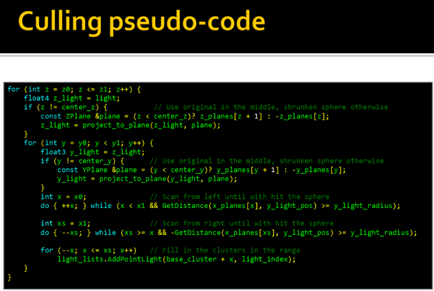 .
.
-
-
Spotlight :
-
For spotlights we begin by finding the ”cube” of clusters around the light’s sphere, just like for pointlights, except this cube typically is much larger than necessary for a spotlight. However, this analytical test is cheap and goes a long way to limit the search space for following passes. Next we find a tighter ”cube” simply by scanning in all six directions, narrowing it down by doing plane-cone tests. There is likely a neat analytical solution here, but this seemed non- trivial. Given that the plane scanning works fine and is cheap we haven’t really explored that path.
-
Note that our cones are sphere-capped rather than flat-capped. That’s because the light attenuation is based on distance (as it should), rather than depth. Sphere-capped cones also generally behave much better for wide angles and doesn’t become extremely large as flat-capped cones can get.
-
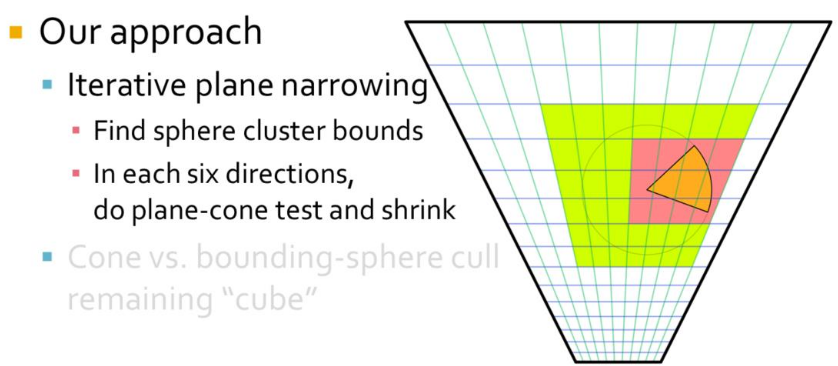
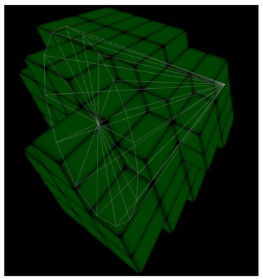 .
.
-
Finally, for the remaining ”cube” of clusters we cull each cluster with a sphere-capped cone vs. bounding sphere test. For this to work well we have to have relatively cubical shaped clusters, otherwise the bounding sphere becomes way oversized. Overall this technique results in a moderately tight culling that is good enough for us so far, although there is room for some minor improvement.
-
-
Shading
-
Shading differs from Tiled Shading only in how we look up the cluster for the view sample in question.
-
For Tiled Shading, a simple 2D lookup, based on the screen-space coordinates, is sufficient to retrieve light-list offset and count. However, for clustered approaches, there no longer exists a direct mapping between the cluster key and the index into the list of unique clusters.
-
In the sorting approach, we explicitly store this index for each pixel. This is achieved by tracking references back to the originating pixel, and, when the unique cluster list is established, storing the index to the correct pixel in a full screen buffer.
-
When using page tables, after the unique clusters are found, we store the cluster index back to the physical memory location used to store the cluster key earlier (using the same page table as before). This means that a virtual lookup for the cluster key will yield the cluster index. Thus, each sample can look up the cluster index using the cluster key computed earlier (or re-computed).
Cluster Key Packing
-
For maximum performance when using sorting or page tables, we wish to pack the cluster key into as few bits as possible. We allocate 8 bits to each i and j components, which identify the screen-space tile the cluster belongs to. This allows up to 8192 × 8192 size render targets (assuming screen-space tile size of 32 × 32 pixels). The depth index k is determined from settings for the near and far planes and Equation 2. In our scenes, we found 10 bits to be sufficient. This leaves up to 6 bits for the optional normal clustering. Using 6 bits, we can for instance support a resolution up to 3 × 3 subdivisions on each cube face (3 × 3 × 6 = 54 and dlog2 54e = 6). For more restricted environments, the data could be packed more aggressively, saving both time and space.
Tile sorting
-
To the cluster key (between 10 and 16 bits wide) we attach an additional 10 bits of meta-data, which identifies the sample’s original position relative to its tile. We then perform a tile-local sort of the cluster keys and the associated meta-data. The sort only considers the up-to 16 bits of the cluster key; the meta-data is used as a link back to the original sample after sorting. In each tile, we count the number of unique cluster keys. Using a prefix operation over the counts from each tile, we find the total number of unique cluster keys and assign each cluster a unique ID in the range
[0...numClusters). We write the unique ID back to each pixel that is a member of the cluster. The unique ID also serves as an offset in memory to where the cluster’s data is stored. -
Bounding volumes (AABB and normal cone) can be re-constructed from the cluster keys, in which case each cluster only needs to store its cluster key. For explicit bounding volumes, we additionally store the AABB and/or normal cone. The explicit bounding volumes are computed using a reduction operation: for instance, AABBs can be found using a min- and a max-reduction operation on the sample positions. The meta-data from the locally sorted cluster keys gives us information on which samples belong to a given cluster.
Shadows
-
Efficient Virtual Shadow Maps for Many Lights - Ola Olsson - 2014 .
-
This paper builds on clustered shading.
-
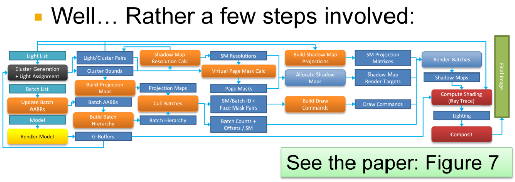 .
.
-
-
Etc :
-
I saw this in some paper and left it loose; maybe I’ll revisit it later.
-
Resolution Matched Shadow Maps (RMSM), must determine which shadow pages are used by the view samples. The method achieves this by first exploiting screen space coherency to reduce duplicate requests from adjacent pixels in screen space. Globally unique requests are then determined by sorting and compacting the remaining requests.
-
Garanzha present a similar technique that they call Compress-Sort-Decompress (CSD). Their goal is to find 3D (or 5D) clusters in a frame buffer, which are used to form ray packets. The main differences are that Garanzha et al. treat the frame buffer as a 1D sequence and use run length encoding (RLE) to reduce duplicates before sorting. They expand the result after the sorting.
-
The approaches in both RMSMs and CSD rely on the presence of coherency between adjacent input elements, in 2D and 1D respectively. In many cases, this is a reasonable assumption. However, techniques such as multi sampling anti aliasing (MSAA) with alpha-to-coverage, or stochastic transparency, invalidate this assumption. Coherency is still present in the frame buffer, but not between adjacent samples. For scenes with low coherence between adjacent samples, both of these methods degenerate to sorting the entire frame buffer.
-
-
It has even been stated that shadow maps are unsuited for many lights. However, when limiting the problem as I have just done, there really is no fundamental reason against shadow maps. And given that they are the de facto standard in the real-time industry, they must clearly be the first stop, if nothing else to provide a benchmark for more clever ideas.
-
To create shadow maps, we need to perform the following steps each frame, using the current camera view:
-
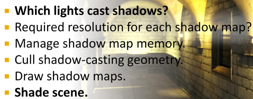 .
.
-
The first step is the same as determining what lights are needed for shading, and we have already seen how this can be achieved using clustered shading and other methods.
-
The last step is also fairly trivial, using bindless textures , array textures or shadow map atlases .
-
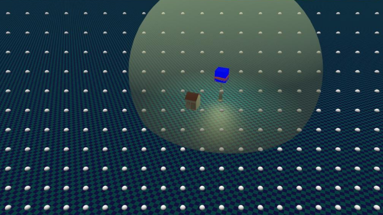
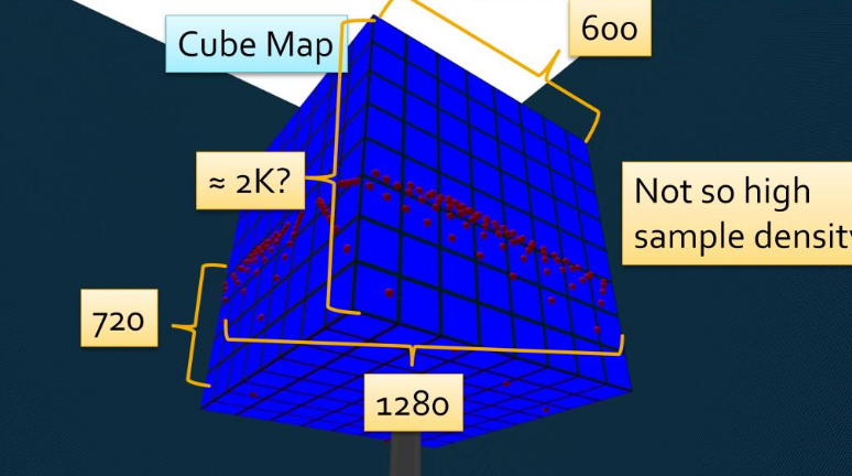 .
.
-
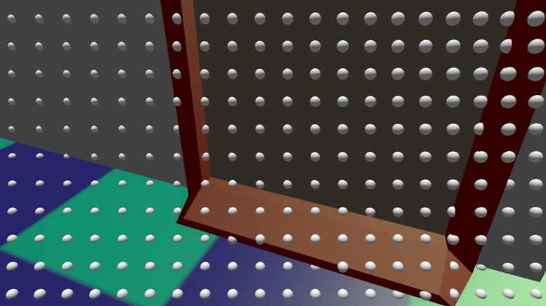
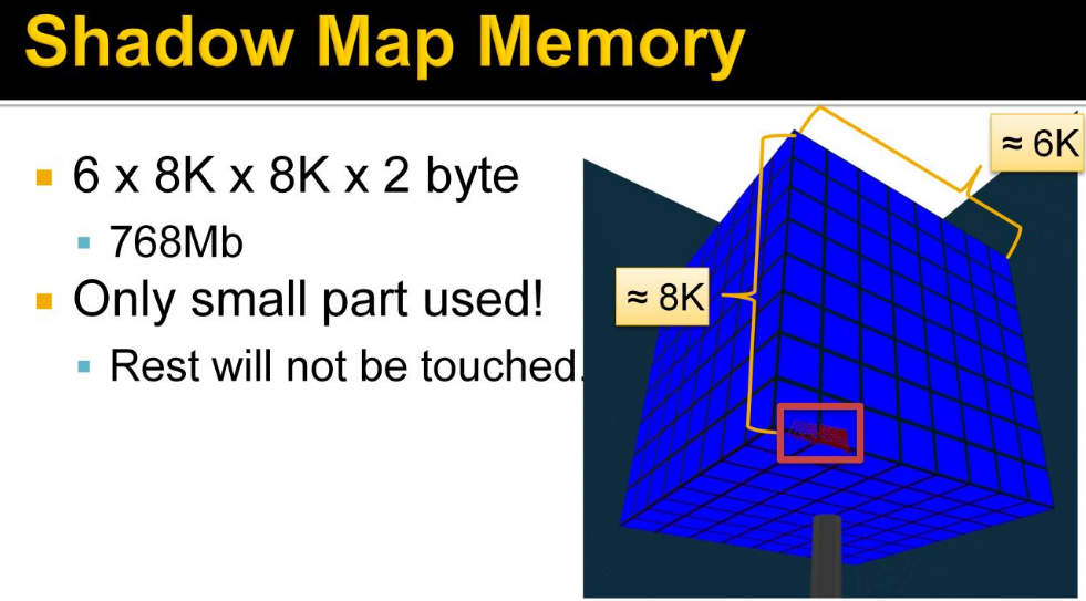 .
.
-
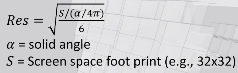 .
.
-
As we saw before, the shadow map samples can be very tightly grouped, requiring a high shadow map resolution And note how this happens when most of the shadow map would be unused! This is pretty much how it has to be, as the high density comes from looking at something very near the camera, and then we’re guaranteed to not see so very much of the scene. This is highly wasteful and a fantastic opportunity, for...
-
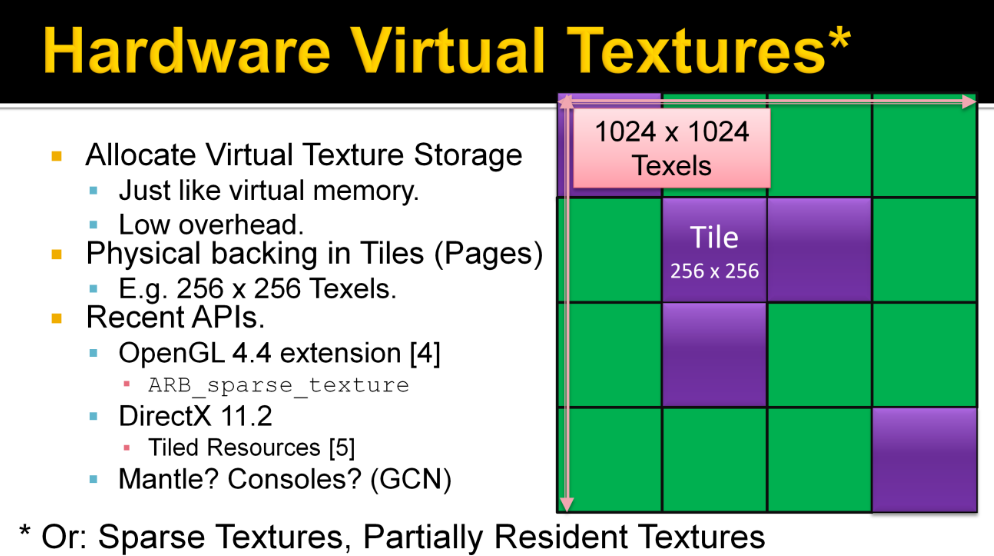 .
.
-
Keyword: Virtual Shadow Maps (Virtual SMs).
-
See pages 181 to 195 of Efficient Real-Time Shading with Many Lights - Ola Olsson, Emil Persson (Avalanche) - 2014 for more information.
-
-
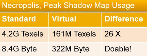 .
.
-
In other terms, this means the difference between impossible on a current console and something we might consider.
-
Our method achieves quite uniform shadow quality, this means we can control quality and thus memory usage with a global parameter. This allows more flexibility in memory use while maintaining uniform quality. An interesting idea is to do this dynamically, to ensure a certain memory budget. Should be possible as it is very quick to work out memory usage from the used pages and resolutions.
-
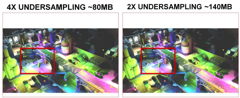
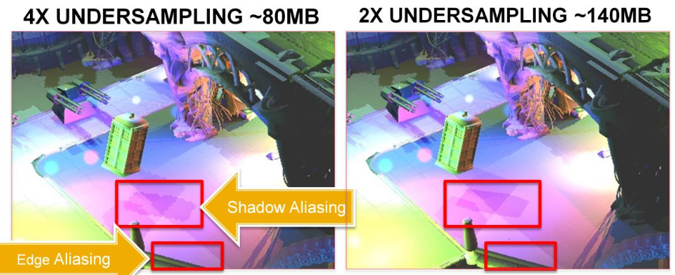 .
.
-
Recall that the peak is 322MB without reducing quality.
-
Cull Shadow Cast Geometry :
-
This process is just like normal view frustum culling, in that we are trying to get rid of geometry that is not visible, and that we do this by testing bounding volumes of chunks or batches of triangles.
-
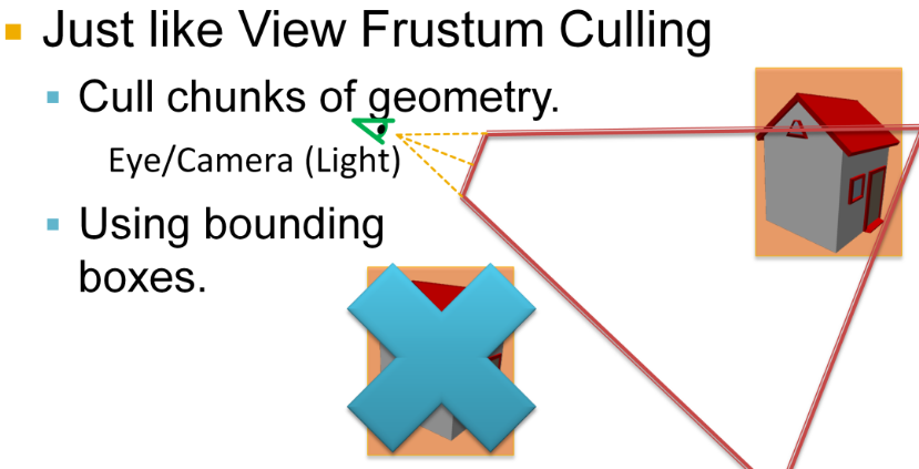
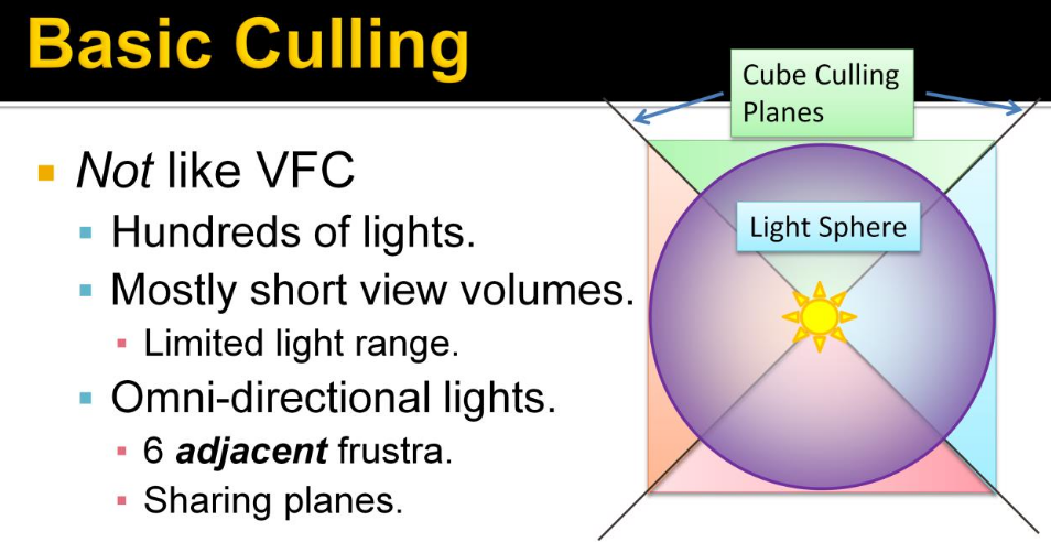 .
.
-
What is not like view frustum culling is that we need to perform hundreds of these tests. The view volumes are quite small, or short, given the limited range of the lights. There are 6 adjacent frustra sharing planes. This adjacency means we can share calculations.
-
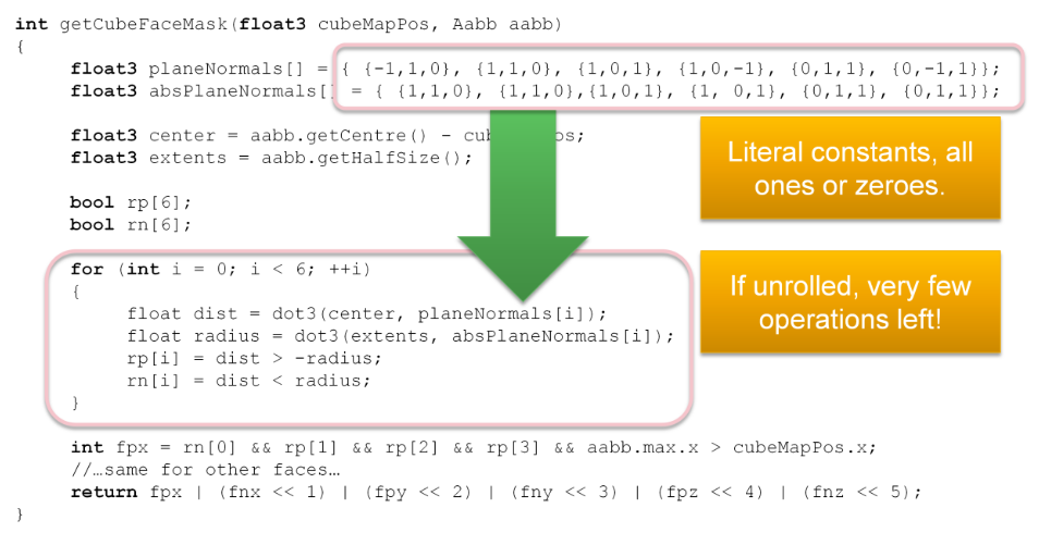 .
.
-
Here is the somewhat condensed code we use to calculate the culling mask, with a bit for each cube face. This is a very efficient test, checking only 6 planes for six frustums. Especially as the plane equations are all ones and zeroes, which means that if the loop is unrolled, most of this code just goes away. I think this is a rather big advantage with cube maps, over using separate frustums (As done in [6]). This efficiency is especially important given that we will be culling a lot more objects than normal culling!
-
You see, to enable efficient culling, batches must be small. Intuitively, for any culling, the optimal size of batches correlates to the size of the frustums. If batches are too large, the triangles get replicated into most cube faces.
-
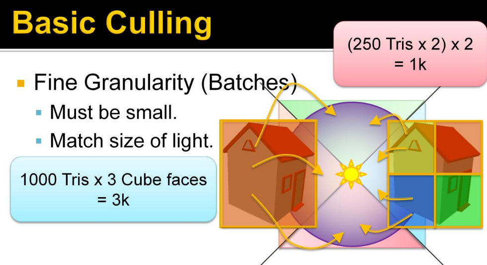 .
.
-
So we are trading increased culling work for fewer triangles drawn. Triangle drawing is the biggest performance bottleneck so this is important to be able to tune.
-
We used batches of up to 128 triangles, in practice they average around 68 triangles. A batch is represented by an AABB and a list of triangles. The batches are constructed in a pre-process, that builds a tree using agglomerative clustering (see the paper section 6.2.1). Note that the quality of the batches is fairly important for good performance. The batches are stored in a flat array that is loaded into the runtime.
-
These values remind me of "clusters in the rabbit". See Optimization Techniques -> Cluster.
-
-
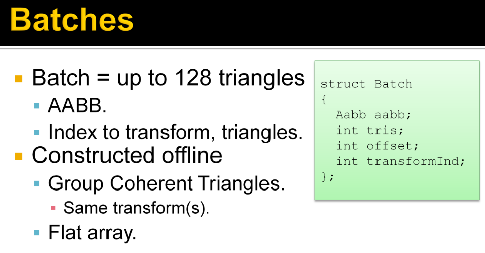 .
.
-
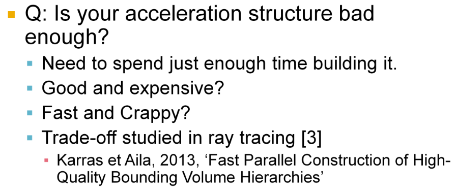 .
.
-
For efficient culling, we obviously need a hierarchy.
-
The important thing is to balance the time spent building and traversing an acceleration structure. This trade-off has been studied by Karras and Aila in context of ray tracing, and is a very interesting read. In short, it suggests to me that the acceleration structure for just a few thousand box queries must be pretty bad to be worth building.
-
We used a very simple, full, 32-way BVH which is completely rebuilt each frame. This is in no way the best possible structure, or even the fastest to build, but it has served us well.
-
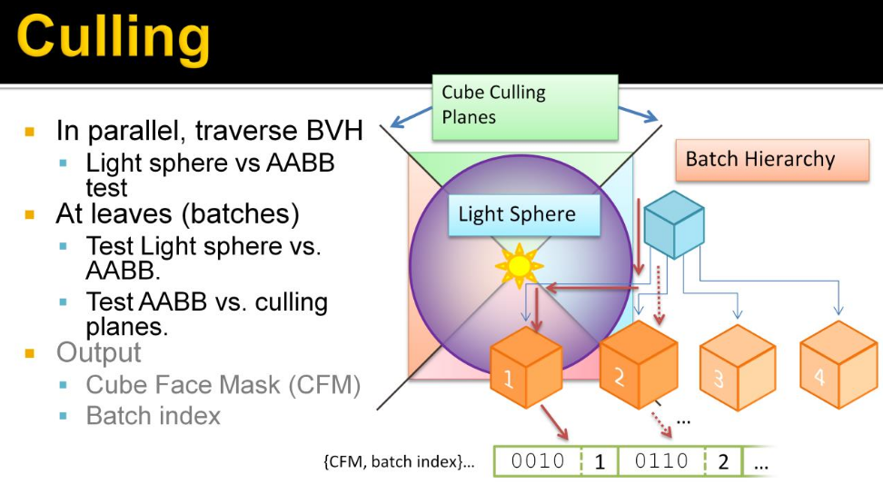 .
.
-
Here we parallelize the lights, and each light traverses the hierarchy to find the batches that overlap the sphere. These batches are those that may produce a shadow if drawn into the shadow map.
-
This produces a list for each light of pairs of cube face masks and batch indexes. The Cube Face Mask is a bit mask where each bit indicates if it overlaps a certain cube face. This tells us what batches to draw to which cube faces of each light.
-
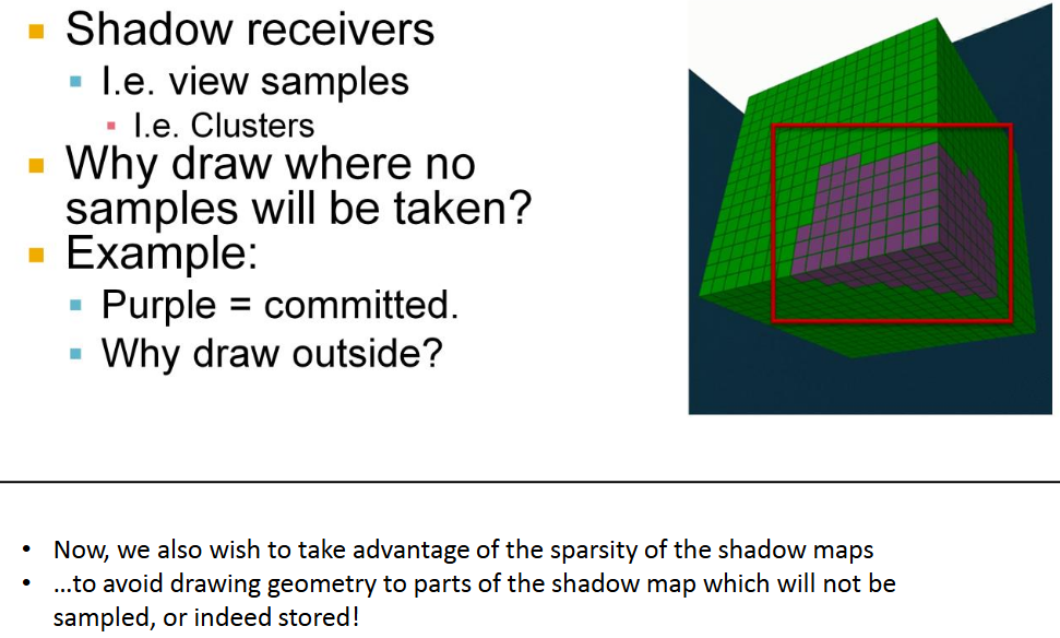 .
.
-
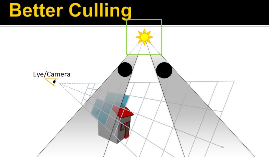 .
.
-
Green: source light BB.
-
Black: Shadow casters.
-
Blue: Clusters containing samples.
-
-
Note that the shadow casters are outside of the view volume, and so have no clusters associated, but cast their shadow through the view volume. So we’re interested in finding out what shadows affect the visible samples, and thus determine if the shadow caster needs to be drawn.
-
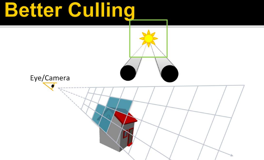 .
.
-
Instead of doing some crazy thing, like shadow volumes, we can figure this out by projecting the shadow caster onto the light source. This gives us these two intervals on the cube face.
-
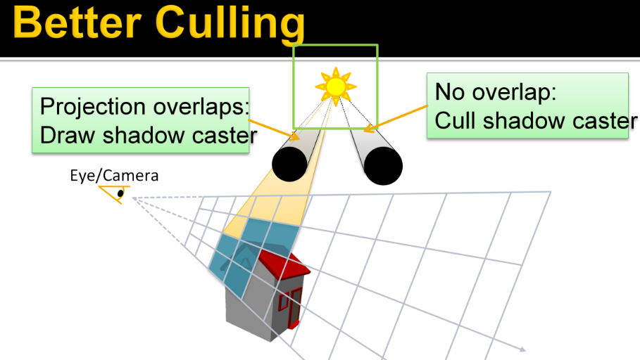 .
.
-
Doing the same thing for the clusters, gives us another interval. If the projection of a shadow caster overlaps that of some clusters, i.e. shadow receiver, …it needs to be rendered into this shadow map, else, it doesn’t. Note that the clusters don’t need to form a range for this to work, any overlap will do.
-
The subject continues from pages 225 to 243 of Efficient Real-Time Shading with Many Lights - Ola Olsson, Emil Persson (Avalanche) - 2014 .
-
I found it quite specific and complicated to implement, for something I'm not focusing on right now.
-
-
-
-
Avalanche Studios :
-
Classic deferred has the advantage that you can iterate light by light, and thus reuse resources such as shadow buffers in between. This saves some memory, which may be needed on current generation consoles. On PC and next-generation consoles this is not nearly as big a problem.
-
With the switch to clustered shading the cost of adding a new light to the scene is small. Artists can now be moderate ”wasteful” without causing much problems performance-wise. This is not true for rasterizing shadow buffers. They remain expensive, and relatively speaking going to be more expensive going forward since it’s often a ROP-bound process, and ROPs aren’t getting scaled up nearly as much as ALU. So we still need to be a bit conservative about how many shadow casting lights we add to the scene.
-
An observation that was made is that artists often place very similar looking lights close to each other. In some cases it is to get a desired profile of a light, in which case the two lights may in fact be centered at the exact same point. But often it is motivated by the real world, such as two headlights on car. Some vehicles actually have ten or more lights, all pointing in the same general direction. Rendering ten shadow buffers for that may prove to be far too expensive.
-
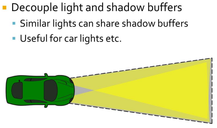 .
.
-
Often it works just fine to share a single shadow buffer for these lights. While the shadow may be slightly off, this is usually not something that you will notice unless you are specifically looking for it. To make this work the shadow buffer is decoupled from lights and the light is assigned a shadow buffer and frustum from which to extract shadows. The shadow frustum has to be large enough to include all the different lights that uses it.
-
Transparency
-
When the transparent geometry is considered, the depth range optimization cannot be fully used. Instead, only a more conventional hierarchical depth test can be used. The grid structure can be built once, and quickly pruned to prepare a more efficient instance for opaque geometry. However, as each transparent layer must consider all the lights in the tile, performance does not scale linearly with the depth complexity, but far worse.
-
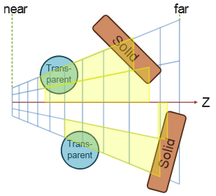 .
.
-
-
To improve on this we extend clustered forward shading by constructing the grid using a pre-pass over all geometry (not just opaque), and flagging clusters as a side effect. This allows us to quickly find the unique clusters used.
-
As clusters contain only space around actual samples that need shading, efficiency is much better.
-
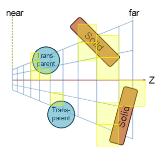 .
.
-
-
For deferred shading a single 1080p, 16x MSAA, 16-bit float RGBA buffer requires over 250Mb of memory. In addition, each sample may need to be shaded individually, effectively running shading at a per-sample frequency.
-
For forward shading, no G-Buffers are required and MSAA is trivially enabled.
Optimized Forward Renderer
-
High-level overview :
-
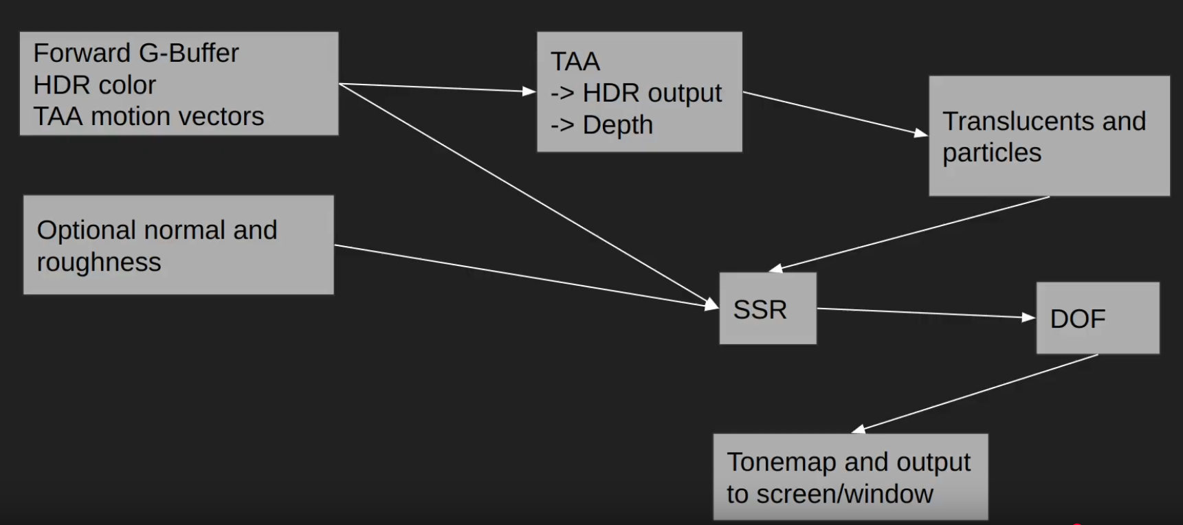 .
.
-
-
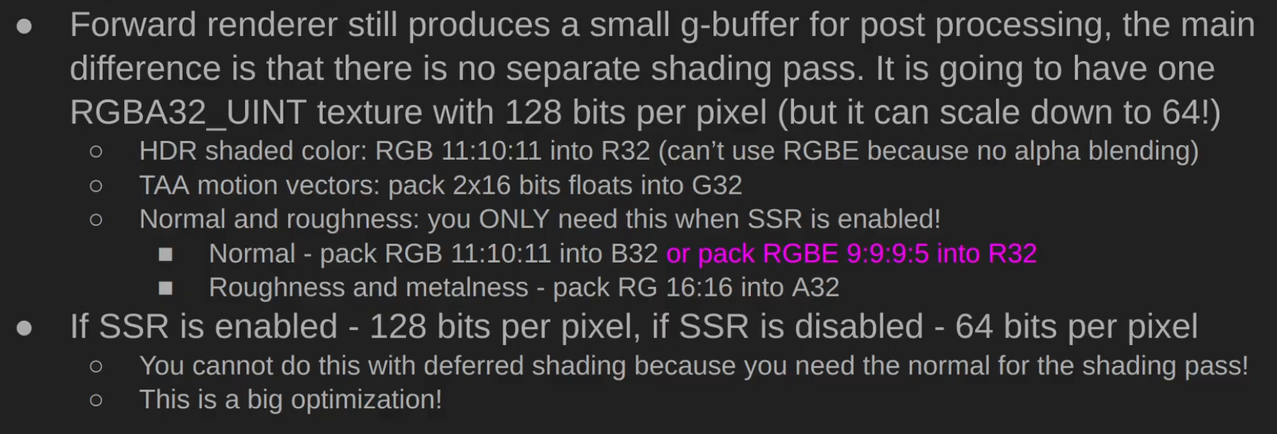 .
.
-
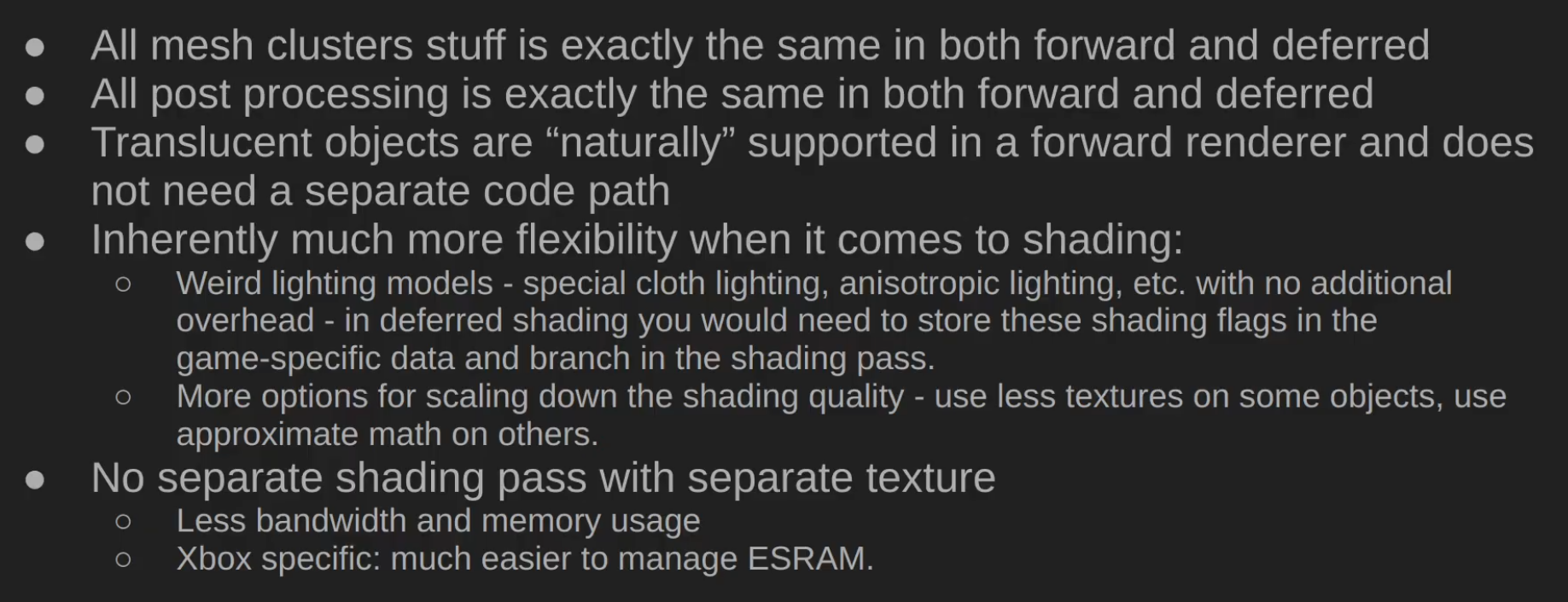 .
.
-
Performance caveats :
-
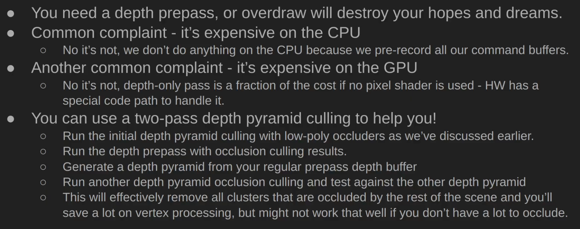 .
.
-
-
Triangle Overshading :
-
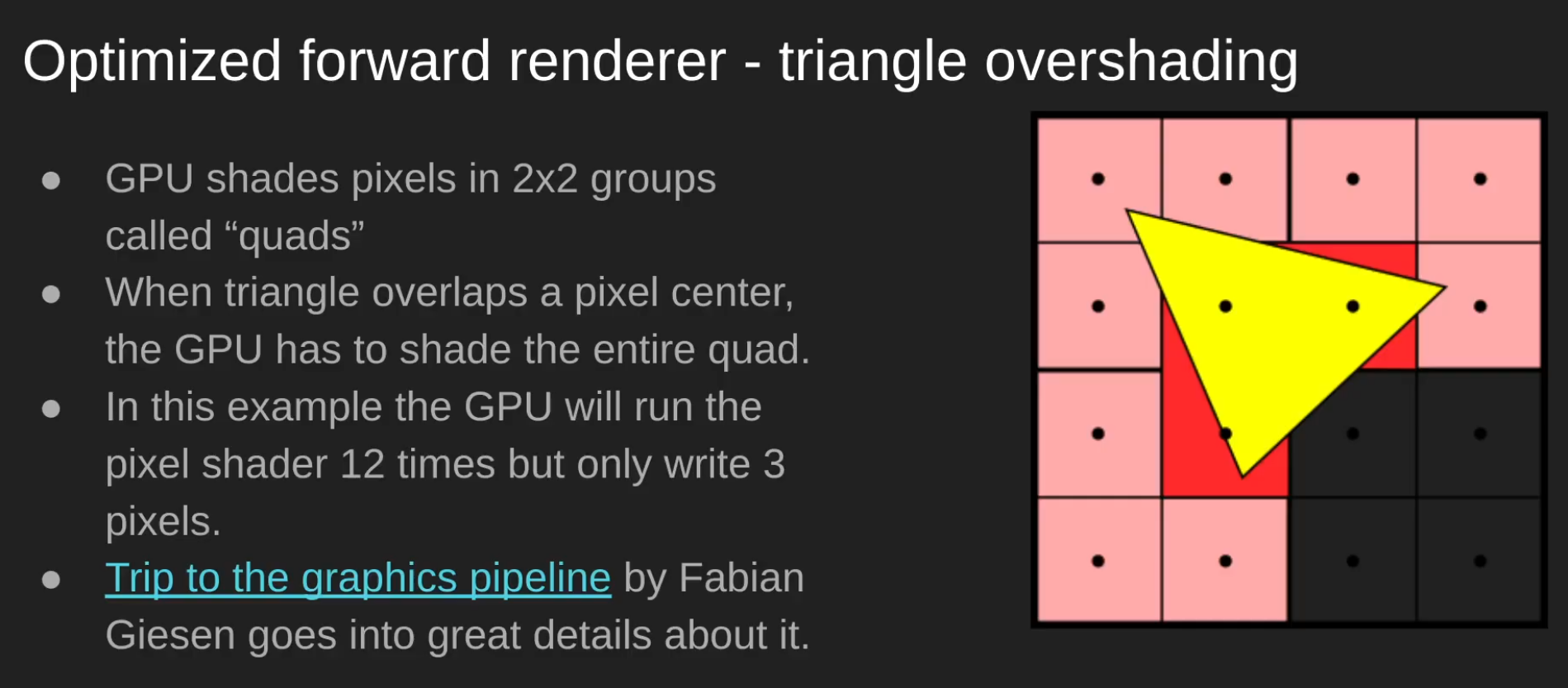 .
.
-
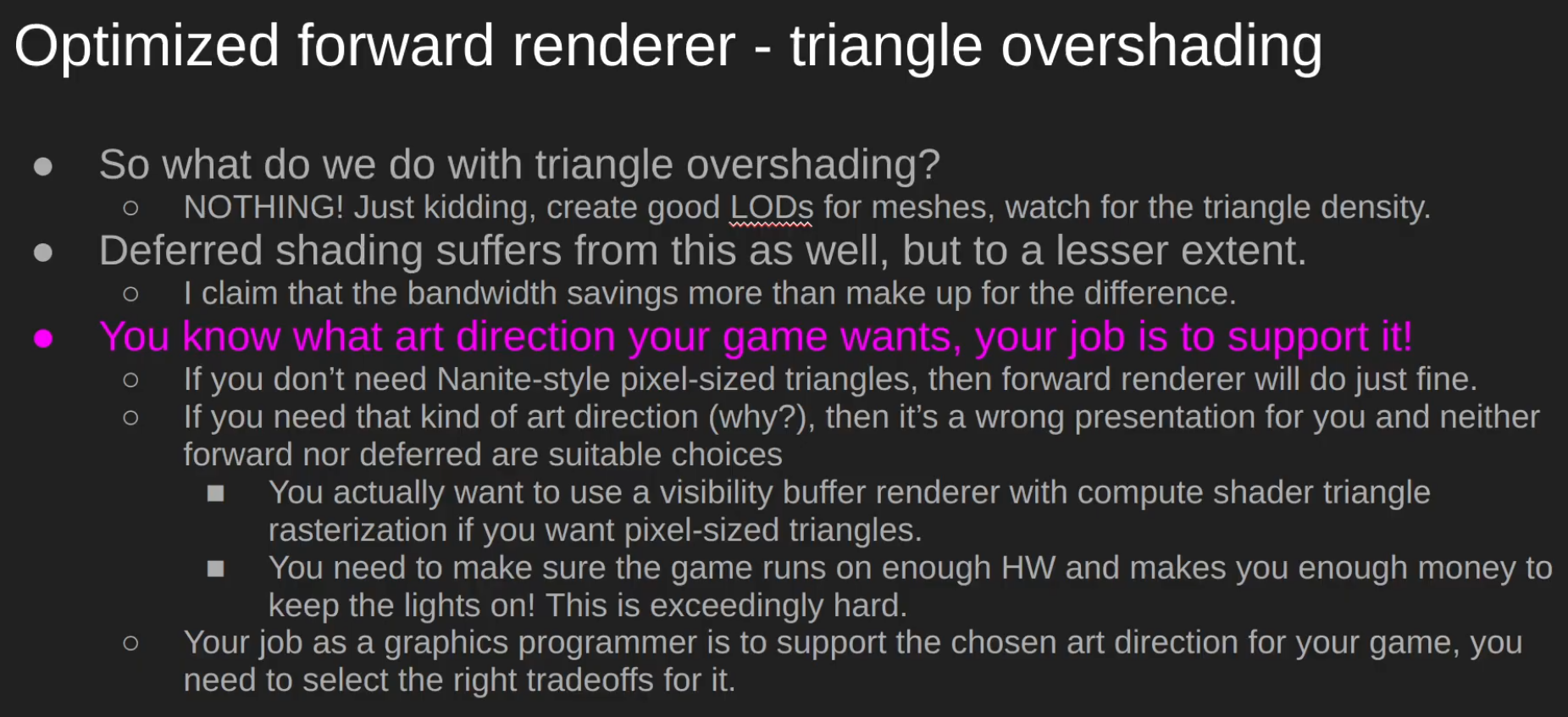 .
.
-
Papers and Presentations
-
Clustered Deferred and Forward Shading - Ola Olsson - 2012 .
-
Tiled and Clustered Forward Shading Supporting Transparency and MSAA - Ola Olsson - 2012 .
-
Efficient Real-Time Shading with Many Lights - Ola Olsson, Emil Persson (Avalanche) - 2014 .
-
Avalanche Studios did:
-
Just Cause 1 (Forward), Just Cause 2 (Forward), Mad Max (Deferred).
-
Just Cause 3, Just Cause 4, Generation Zero, Rage 2.
-
-
-
A Primer On Efficient Rendering Algorithms & Clustered Shading - Angel Ortiz - Rockstar North - 2018 .
-
Part 2 explains the implementation of the technique.
-
Great read, pretty good, with some implementation explanations and source code in OpenGL.
-
-
Cluster Shading OpenGL - David Hu - 2024 .
-
This is not a sample, just a C++ and OpenGL tutorial with some GLSL shaders for reference.
-
-
Clustered Forward Rendering and Anti-Aliasing in Detroit: Become Human - GDC 2018 .
-
~ Volume Tiled Forward Shading - Jeremiah Van Oosten - 2017 .
-
Supposedly: Volume > Clustered > Tiled.
-
Volume Tiled Forward Shading is based on Tiled and Clustered Forward Shading from Ola Olsson.
-
By first constructing a Bounding Volume Hierarchy (BVH) over the lights, we can achieve millions of light sources while maintaining real-time frame rates.
-
Impressions :
-
So... it seems the only thing he did was add BVH to the technique, however that seems to already be done by default in the culling part of Clustered Shading....
-
I don't understand. Did someone copy someone here? I'm confused...
-
His master's thesis is huge, but much of it is kind of "padding", as it's just a presentation of previous works.
-
Hmmm idk. He's not wrong, it just sounds odd.
-
-
-
Practical Clustered Shading - Avalanche Studios 2015.-
Exactly the same presentation as 'Efficient Real-Time Shading with Many Lights - Ola Olsson, Emil Persson (Avalanche) - 2014'; see that presentation, since it has presenter comments.
-
-
Practical Clustered Shading 2/4 - Avalanche Studios - 2014.-
The presentation comes after 'Efficient Real-Time Shading with Many Lights - Ola Olsson, Emil Persson (Avalanche) - 2014', since Just Cause 3 had already been announced, using Clustered Shading.
-
The presentation is very similar to 'Efficient Real-Time Shading with Many Lights - Ola Olsson, Emil Persson (Avalanche) - 2014'.
-
-
Managing many lights in real time with clustered shading - Ola Olsson 2016.-
Based on the 'Efficient Real-Time Shading with Many Lights - Ola Olsson, Emil Persson (Avalanche) - 2014' presentation, with basically no changes.
-
I preferred to read the former, for better slide visibility and because the presentation is much more in-depth. Also, the earlier presentation seemed to have more enthusiasm and depth; perhaps the audience for this presentation did not show much enthusiasm.
-
Samples
-
HybridRenderingEngine OpenGL (Clustered Forward/Deferred) - Sample - Angel Ortiz - 2018 .
-
Clustered Forward/Deferred Renderer
-
Physically Based shading
-
Image Based Lighting
-
Metallic workflow
-
Cook-Torrance specular BRDF (w/ lambert diffuse)
-
Ambient Occlusion & Emissive mapping
-
Tangent space normal mapping
-
HDR/linear lighting
-
HDR/LDR skyboxes
-
Exposure based tone mapping
-
Bloom
-
Multisample Anti-aliasing (MSAA)
-
Directional & point light sources
-
Compute shader based light culling
-
Alpha tested foliage (sponza atrium)
-
Directional light dynamic shadow mapping
-
Static Omnidirectional Shadow Mapping for Point Lights
-
Forward, Tiled Forward and Deferred rendering implementations
-
Located in other branches of the repo. Only clustered rendering is actively being developed.
-
-
Engine:
-
OpenGL 4.5+
-
SDL2 backend
-
JSON Parsing via Nlohmann: JSON for C++
-
Model Loading via ASSIMP (OBJ, FBX, gLTF2.0 etc)
-
Scene contents clearly outlined in JSON file
-
Multiple image loading paths via stb-image and GLI
-
Immediate mode GUI for debugging via ImGUI
-
Fully commented for future referencing
-
Environment map generation on load for IBL and skyboxes
-
Free flight camera
-
-
Deferred Shading
Deferred
-
Deferred shading is a screen-space shading technique that is performed on a second rendering pass, after the vertex and pixel shaders are rendered.
-
"I like to call it a "fake rendering", as at the end of the day you'll be just doing your shading on a quad, not on the geometry".
-
A shader that collects all geometry information into buffers, matches the first stage of a deferred renderer.
-
GBuffer ("Geometry Buffer") :
-
G-buffer is a set of textures or render targets used in deferred shading/rendering.
-
Instead of directly shading fragments during rasterization (as in forward rendering), the GPU first stores per-fragment data into the G-buffer.
-
A later pass (the lighting pass) reads from these buffers to compute lighting, shadows, reflections, etc.
-
A typical G-buffer contains attributes such as:
-
World/eye space position of the fragment
-
Normals
-
Albedo (base color)
-
Specular properties
-
Possibly depth, roughness, metalness, etc.
-
-
The key point is: the first pass writes geometry information into multiple render targets (the G-buffer), and the second pass consumes it for lighting.
-
-
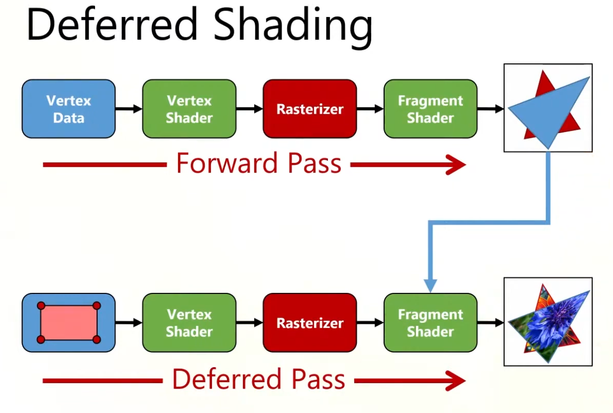 .
.
-
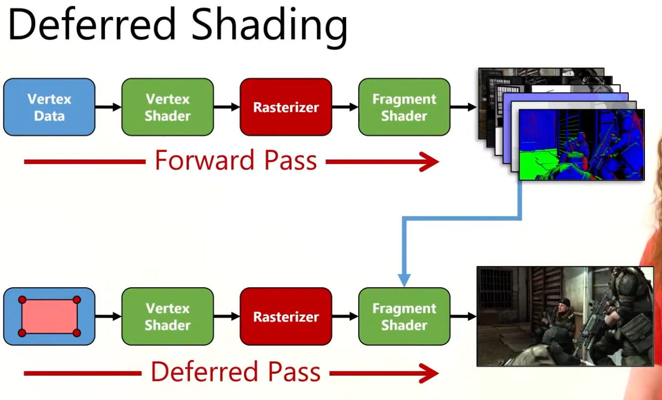 .
.
-
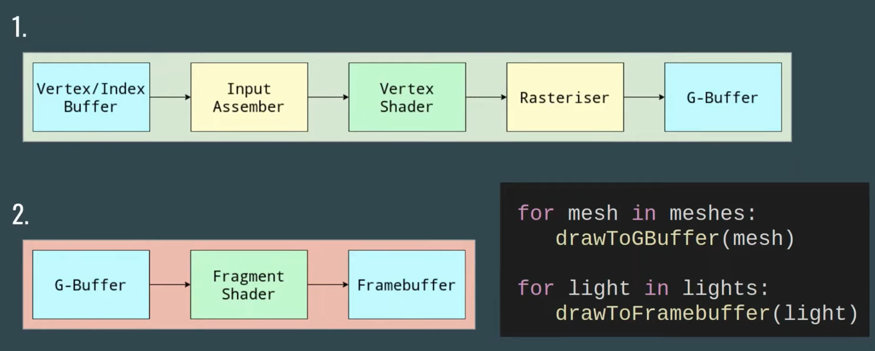 .
.
-
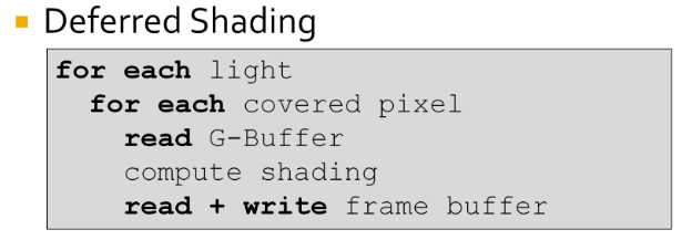 .
.
-
The problem is from the fact that the innermost loop is over the pixels.
-
This requires repeated reading and writing of the G-Buffers and frame buffer.
-
Disadvantages
-
Bandwidth :
-
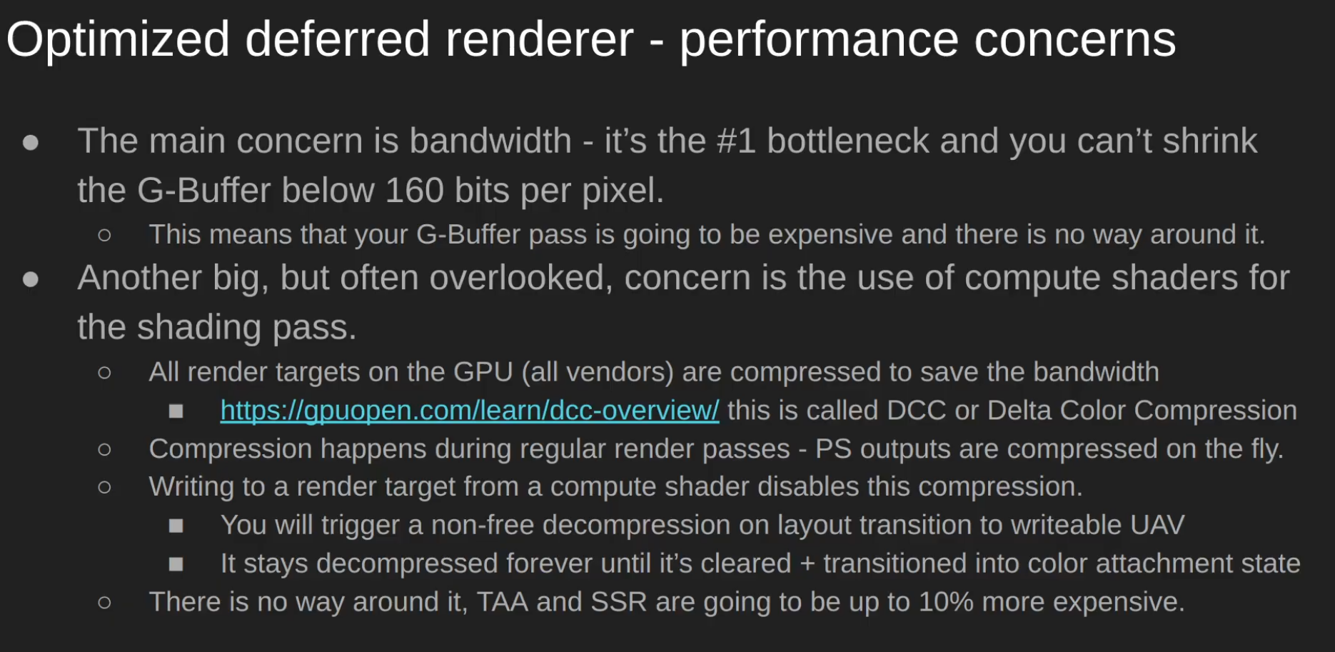 .
.
-
Consider marking non-persistent attachments as transient (
VK_ATTACHMENT_STORE_OP_DONT_CARE/ lazily allocated) so tile-based GPUs can keep them on-tile and reduce bandwidth.
-
-
Transparency :
-
Inability to handle transparency within the algorithm, although this problem is a generic one in Z-buffered scenes and it tends to be handled by delaying and sorting the rendering of transparent portions of the scene.
-
Depth peeling can be used to achieve order-independent transparency in deferred rendering, but at the cost of additional batches and g-buffer size.
-
Modern hardware, supporting DirectX 10 and later, is often capable of performing batches fast enough to maintain interactive frame rates.
-
When order-independent transparency is desired (commonly for consumer applications) deferred shading is no less effective than forward shading using the same technique.
-
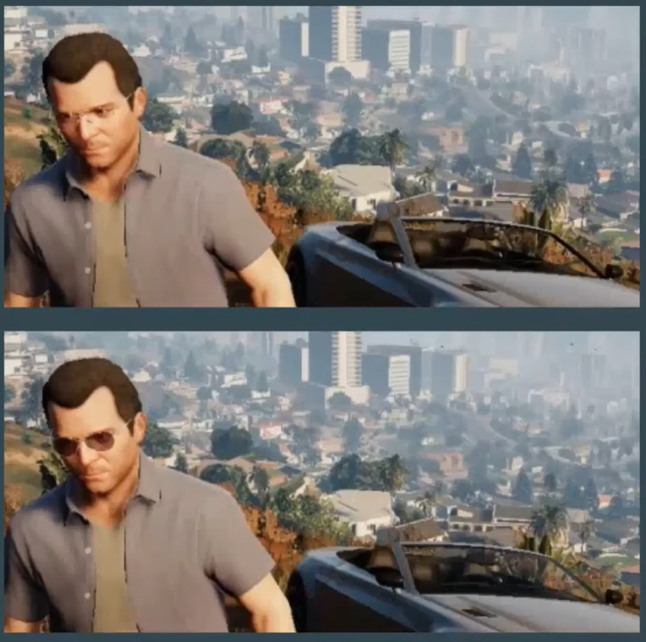 .
.
-
Example from GTA V.
-
-
Opaque is drawn with deferred renderer.
-
Transparent is drawn with forward renderer and then blended with the result of the deferred renderer.
-
-
Difficulty with using multiple materials :
-
It's possible to use many different materials, but it requires more data to be stored in the G-buffer, which is already quite large and takes up a large amount of the memory bandwidth.
-
Memory and bandwidth heavy (multiple render targets).
-
-
Another disadvantage of deferred shading is that only a single lighting model can be simulated in the lighting pass. This is due to the fact that it is only possible to bind a single pixel shader when rendering the light geometry. This is usually not an issue for pipelines that make use of übershaders as rendering with a single pixel shader is the norm, however if your rendering pipeline takes advantage of several different lighting models implemented in various pixel shaders then it will be problematic to switch your rendering pipeline to use deferred shading.
-
Bad MSAA :
-
Due to separating the lighting stage from the geometric stage, hardware anti-aliasing (MSAA) does not produce correct results anymore since interpolated subsamples would result in nonsensical position, normal, and tangent attributes.
-
One of the usual techniques to overcome this limitation is using edge detection (MLAA, FXAA, DLAA, or post MSAA) on the final image and then applying blur over the edges. TAA can also be used.
-
DirectX 10 introduced features allowing shaders to access individual samples in multi-sampled render targets (and depth buffers in version 10.1), giving users of this API access to hardware anti-aliasing in deferred shading. These features also allow them to correctly apply HDR luminance mapping to anti-aliased edges, where in earlier versions of the API any benefit of anti-aliasing may have been lost.
-
-
Extra complexity
-
G-buffer packing, formats, reconstructing positions, light culling systems, extra render passes and descriptor management.
-
Variants
-
As said by Ola Olsson:
-
Deferred Lighting
-
Factor out specular and diffuse color.
-
G-Buffer only stores normal and shininess.
-
Output diffuse and specular shading.
-
Second geometry pass which multiple colors.
-
-
Light Prepass.
-
Much like the above.
-
But with monochromatic specular highlight.
-
-
They offer similar performance as deferred.
-
Only improves constant factors.
-
Limits shading model even further.
Tiled Deferred
-
Tiled deferred shading removes the bandwidth bottleneck from deferred shading, instead making the technique compute bound. This enables efficient usage of devices with a high compute-to-bandwidth ratio, such as modern consoles and GPUs. Modern high-end games are using tiled deferred shading to allow for thousands of lights, which are required to push the limits of visual fidelity.
-
With large numbers of lights, GI effects can be produced that affect dynamic as well as static geometry.
-
Steps:
-
Render scene to G-Buffers.
-
Cluster assignment.
-
Find unique clusters.
-
Assign lights to clusters.
-
Shade samples.
-
-
The first step, rendering the model to populate the G-Buffers, does not differ from traditional deferred shading or from tiled deferred shading. The second step computes for each pixel which cluster it belongs to according to its position (possibly normal). In the third step, we reduce this into a list of unique clusters. The fourth step, assigning lights to clusters, consists of efficiently finding which lights influence which of the unique clusters and produce a list of lights for each cluster. Finally, for each sample, these light lists are accessed to compute the sample’s shading.
-
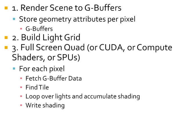 .
.
-
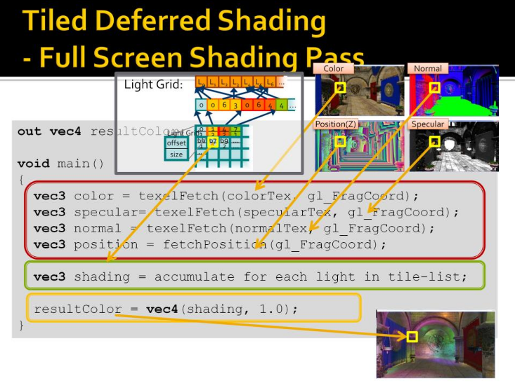 .
.
-
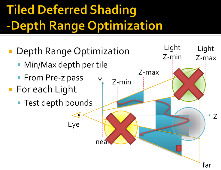 .
.
-
Tiles in 1D, from side
-
View Frustum
-
4 subdivisions
-
Redline is geometry
-
Min and max depth per tile
-
Light range, rejected, completely hidden
-
Another rejected, completely in front
-
Rejected in one tile, not others
-
Usage
-
Uncharted: Drake’s fortune.
-
Battlefield 3.
-
PlayStation 3.
-
Xbox 360.
Optimized Deferred Renderer
-
High-level overview :
-
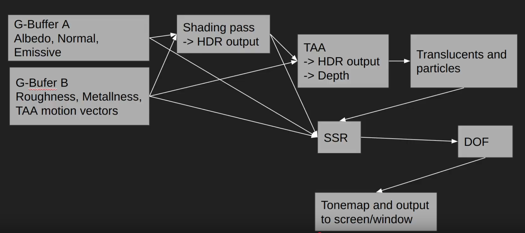 .
.
-
For SSR you need to take a lot of samples from G-Buffer B, and one sample from the shading color from the TAA pass.
-
We do the Raymarching using roughness and depth, once that is done we sample the TAA to get the final color.
-
-
DOF: Depth of Field.
-
-
-
Compressing the GBuffer
-
Optimized deferred shading renderer:
-
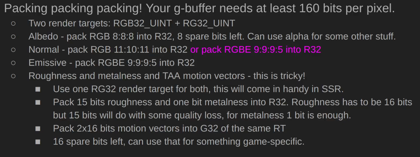 .
.
-
Random person in the comments: There's a small typo - Normal should be G32 and Emissive should be B32.
-
Does it make sense? maybe?
-
-
-
-
Lights :
-
 .
.
-
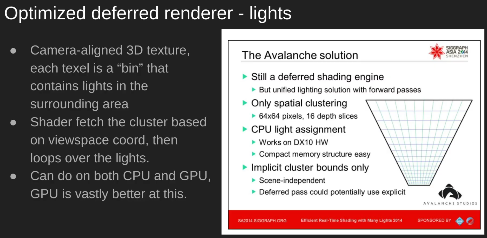 .
.
-
-
Decals :
-
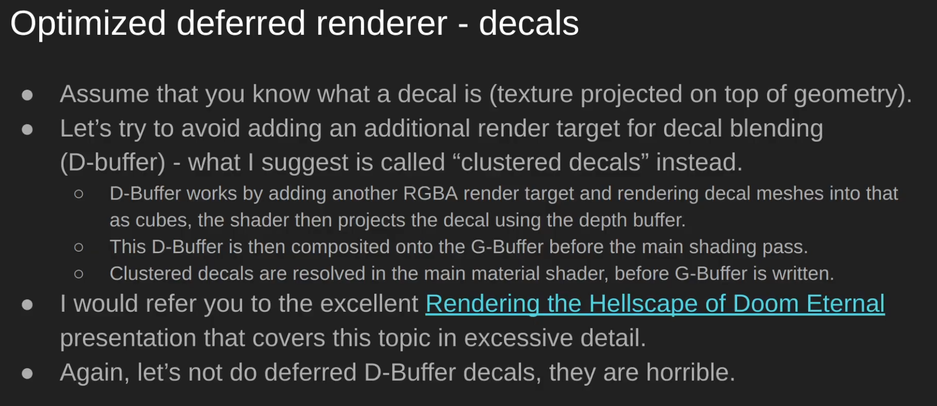 .
.
-
Clustered Decals > D-Buffer.
-
-
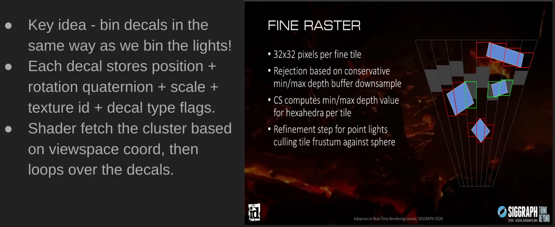 .
.
-
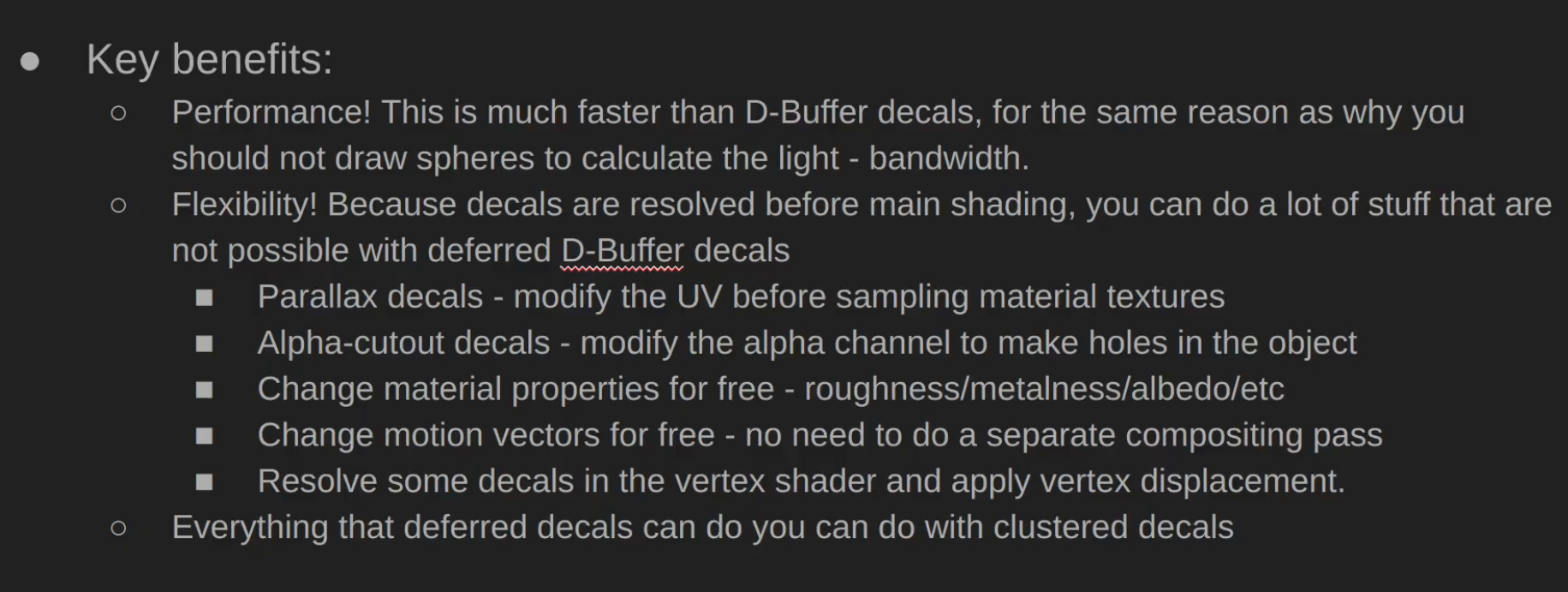 .
.
-
-
Post-processing :
-
 .
.
-
-
Demo and Source Code - Sascha Willems .
-
Based on my deferred shading example this new example adds shadows from multiple spotlights using shadow mapping. To avoid having multiple render passes for rendering the scene's depth from each of the light's point-of-view the example uses a layered depth attachment and multiple geometry shader invocations, so that an arbitrary number of depth maps can be generated in one pass. Each layer in the attachment corresponds to a light source and the geometry shader does multiple invocations on each vertex to output the scene into the different layers of the attachment. Each invocation uses a different light's mvp matrix. The final scene compositing pass then samples from the depth map array texture to determine if a fragment is shadowed or not.
-
-
Demo .
-
"Deferred lighting is physically based, using Cook-Torrance as the BRDF. In this demo the forward pass is only responsible for drawing the skybox, but could draw other rasterization pipelines not suitable for the deferred passes."
-
-
Demo .
-
Jonathan Blow's criticisms of Deferred Rendering .
-
He bullshits and claims it's bad, unjustifiable.
-
"Doesn't make sense in the modern day".
-
Counter-argument:
-
Deferred is defined very very simply - do you have a G-buffer? If the answer is yes - you're deferred.
-
Pretty much all of high-performance forward renderers do a "depth pre-pass", which is sort-of like "deferred lite".
-
Forward has a huge benefit of being very bandwidth efficient, but it's very compute inefficient.
-
About transparencies - transparency is hard. Most forward renderers suck at transparency, most deferred suck as well. Forward makes it a bit easier, because your architecture is about the same.
-
About lighting, Jonathan Blow clearly is not a graphics engineer, there's tiled and clustered rendering that has existed since late 2000s which is typically called Forward+, same techniques are used in deferred, but hey man... the whole lighting argument is over a decade out of date.
-
-
Counter-argument:
-
Deferred solves the problem of doing the pricey per-pixel calculations only on the pixels that will be visible in the end result. Which is why, contrary to what he said, basically every engine went deferred. I like the guy but this is maybe the worst take that I've ever heard him say? He doesn't really get why it's used AND he is wildly off the mark about its popularity in general. If anything, forward had a pretty big comeback with phones and VR.
-
-
Pro argument:
-
Deferred rendering is an optimization technique to make lighting cheaper, but has massive complexity, VRAM, and image quality downsides. There's not really an upside besides being cheap to process many lights. There's a few ultra high end games that are slowly ditching deferred for forward+ systems. I think in a few years there's a good chance deferred won't be common. Even if raytracing doesn't happen.
-
-
Counter-argument:
-
Forward+ still doesn't solve the problem of shadow casting lights. Deferred at least has lower overhead, so the bits of computing power go to shadow mapping purposes.
-
-
Clustered Deferred
-
Avalanche Studios :
-
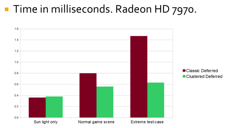 .
.
-
Adaptive Deferred Shading
-
It's a selective way to choose what to perform shading on.
-
He compared it with VRS while using deferred shading.